CS6250 - Computer Networks - Notes

Lesson 1 - Introduction, History, and Internet Architecture

History of the internet

The internet began as many things in tech did, from DARPA.

Specifically:

1. J.C.R. Licklider proposed the “Galactic Network” (1962)
   • Attached a computer in Stanford to a computer at MIT, thus beginning computers talking to each other
2. The ARPANET (1969)
   • UCSB, UCLA, Stanford, and U of Utah interlink
3. Network Control Protocol (NCP), an initial ARPANET host-to-host protocol (1970)
   • The first protocol was designed to handle increasing number of computers, first app built on this was email
4. Inter-networking and TCP/IP (1973)
   • NCP became TCP/IP, IP for addressing and forwarding packets, TCP for flow control and recovery from lost packets
5. The Domain Name System (DNS) (1983) and the World Wide Web (WWW) (1990)
   • As the internet exploded with content and endpoints, they needed a way to turn domains into IP addresses. In walks DNS.

Internet Architecture

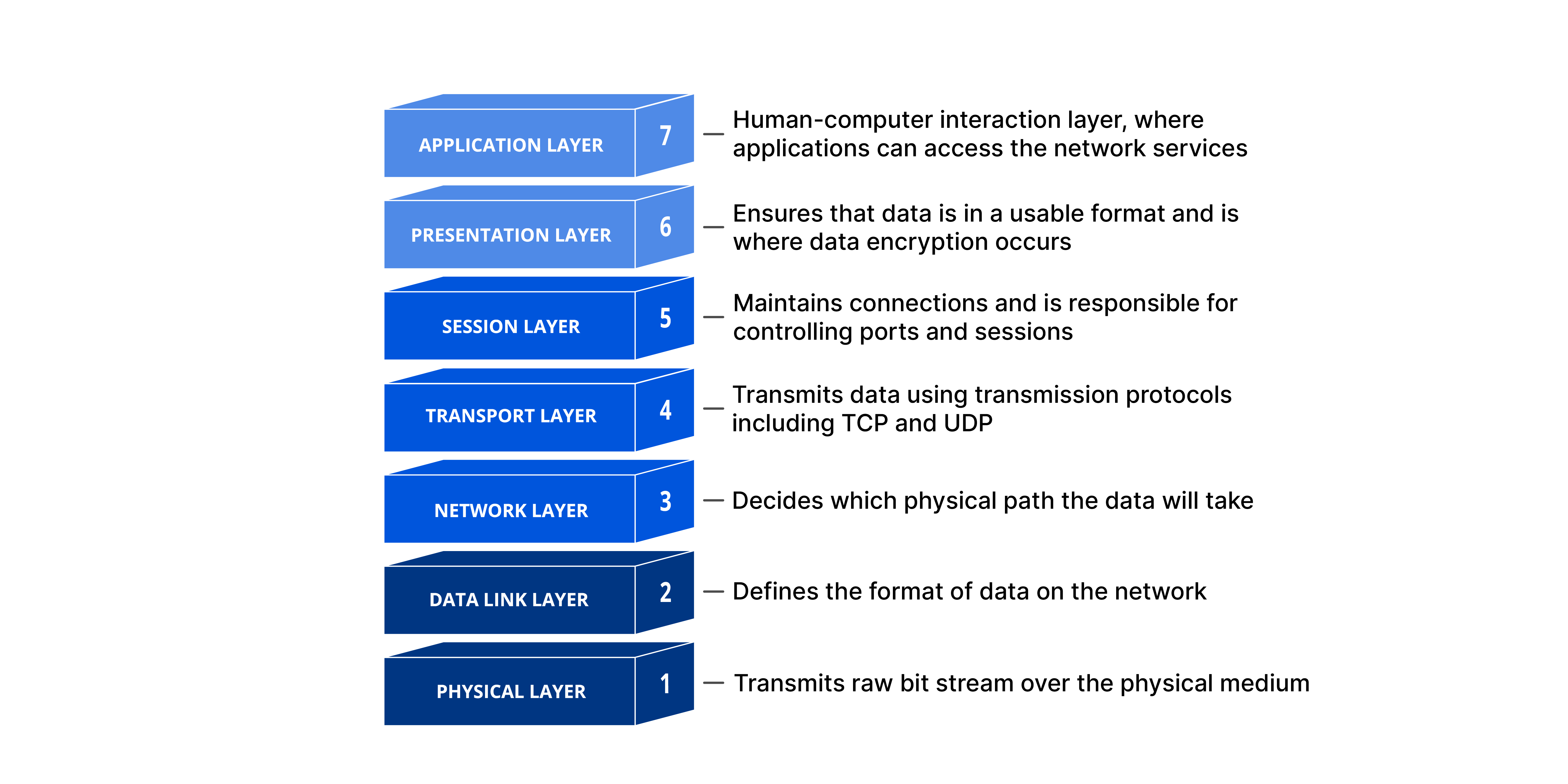
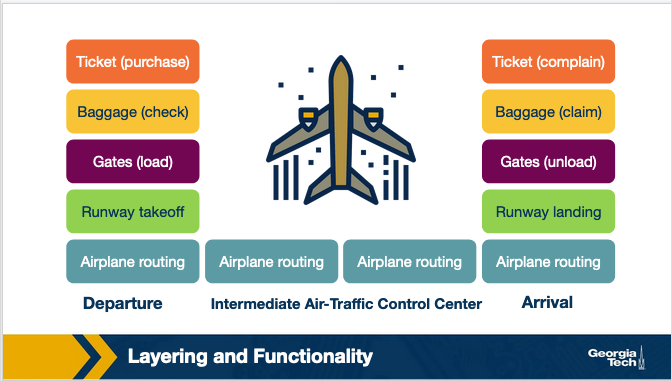
The internet was built in layers. Each layer is supposed to have its own job, and not rely on any of the layers above or below it.

Think of a person as a bit of data, then watch them fly from one airport to another and you get the idea.

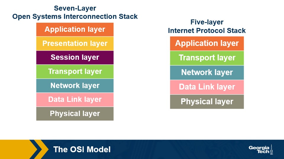
So there is an originally designed theoretical layer named the OSI model, which had 7 layers, and then the layers that were actually implemented, known as the Internet Protocol Stack.

These layers are not as perfect as we would hope, specifically sometimes they do rely on the other layers or they both have methods of solving the same problem like error recovery.

Notice that the Session and Presentation layers disappear in the Internet Protocol Stack, those are handled in the ports of each network device. The logic that is accomplished in those layers still happens, just all in one place.

Application Layer

The data here is a message.

This is the layer we all interact with all the time.

• HTTP (web)
• SMTP (e-mail)
• FTP (transfers files between two end hosts)
• DNS (translates domain names to IP addresses)

Takes the content that we want to ship around, and does all the encoding and decoding needed to actually USE it.

The Presentation Layer

The presentation layer plays the intermediate role of formatting the information that it receives from the layer below and delivering it to the application layer. For example, some functionalities of this layer are formatting a video stream or translating integers from big endian to little endian format.

The Session Layer

The session layer is responsible for the mechanism that manages the different transport streams that belong to the same session between end-user application processes. For example, in the case of a teleconference application, it is responsible to tie together the audio stream and the video stream.

The Transport Layer

The data here is a segment.

End to End communication between hosts.

• Transmission Control Protocol (TCP)
• User Datagram Protocol (UDP)

TCP is better connection-oriented services, guarantees delivery, manages flow control, and controls congestion. This is the USPS, slow but reliable (except TCP doesn’t lose mail like the USPS).

UDP is fast and guarantees nothing. Receivers and Senders using UDP must be able to handle segments getting dropped, delayed, or not making it entirely. But they should be faster when everything is working compared to TCP.

The Network Layer

The data here is a datagram.

This is where IP comes into play. This layer is responsible for connecting one computer to another, via the IP address that everyone has.

The Data Link Layer

The data here is a frame.

This layer is responsible for moving the frames from one node (host or router/switch) to the next node. This uses things like:

1. Ethernet
2. Point-to-point Protocol (PPP)
3. Wi-Fi

The Physical Layer

The actual hardware translation. Translating electricity into bits based on ethernet, coax, fiber, etc.

Encapsulation

These layers work on the idea of encapsulation and de-encapsulation. So encapsulation is to take a chunk of data, package it up, add a header to it and pass it on. Then de-encapsulation is using the headers to decode each chunk of data, until all you’re left with is the data/message.

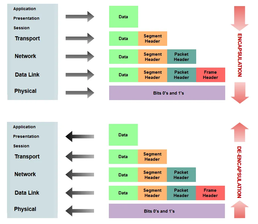
This method is what allows people to build upon the existing infrastructure of the internet, but still make new things.

The End to End (e2e) Principle

The e2e principle shaped the internet as we know it today.

Essentially the principle is that 99% of the complexity should be at the ends of the communications. This allows the underlying infrastructure to be simple, but expandable, and allows people working at the different ends to iterate and create new things quickly.

If they had to change the underlying architecture every time they wanted to change anything it would bring development speed to a crawl.

Beneficial excerpt from the lecture:

Many people argue that the e2e principle allowed the internet to grow rapidly because evolving innovation took place at the network edge, in the form of numerous applications and a plethora of services, rather than in the middle of the network, which could be hard to modify later.

What were the designers’ original goals that led to the e2e principle?

Moving functions and services closer to the applications that use them increases the flexibility and the autonomy of the application designer to offer these services to the needs of the specific application.

Thus, the higher-level protocol layers are more specific to an application. Whereas the lower-level protocol layers are free to organize the lower-level network resources to achieve application design goals more efficiently and independently of the specific application.

Violations of e2e

All rules are meant to be broken.

Firewalls, NAT boxes, and traffic filters all break the e2e principle, and usually for good reason.

NAT routers provide a way to make up for the fact that there aren’t that many IP addresses available in IPv4. Instead of EVERY device having its own worldwide public IP address, you give your home 1 IP address, and then every device behind that has its own local address.

This means that whenever a message is sent to your PC it goes:

Web > Router (Public IP)> End Device (local IP)

The router is breaking some rules of e2e, because it is intervening and inspecting data.

This is the notes’ reasoning for why:

Why do NAT boxes violate the e2e principle? The hosts behind NAT boxes are not globally addressable or routable. As a result, it is not possible for other hosts on the public Internet to initiate connections to these devices. So, if we have a host behind a NAT and a host on the public Internet, they cannot communicate by default without the intervention of a NAT box. Some workarounds allow hosts to initiate connections to hosts that exist behind NATs. For example, Session Traversal Utilities for NAT, or STUN, is a tool that enables hosts to discover NATs and the public IP address and port number that the NAT has allocated for the applications for which the host wants to communicate. Also, UDP hole punching establishes bidirectional UDP connections between hosts behind NATs.

The Hourglass Shape of the Internet

The internet is curvy.

No really, there’s a ton on each end of it, but the middle is pretty narrow. Specifically, TCP, UDP, IP are really the backbone of literally everything. See below:

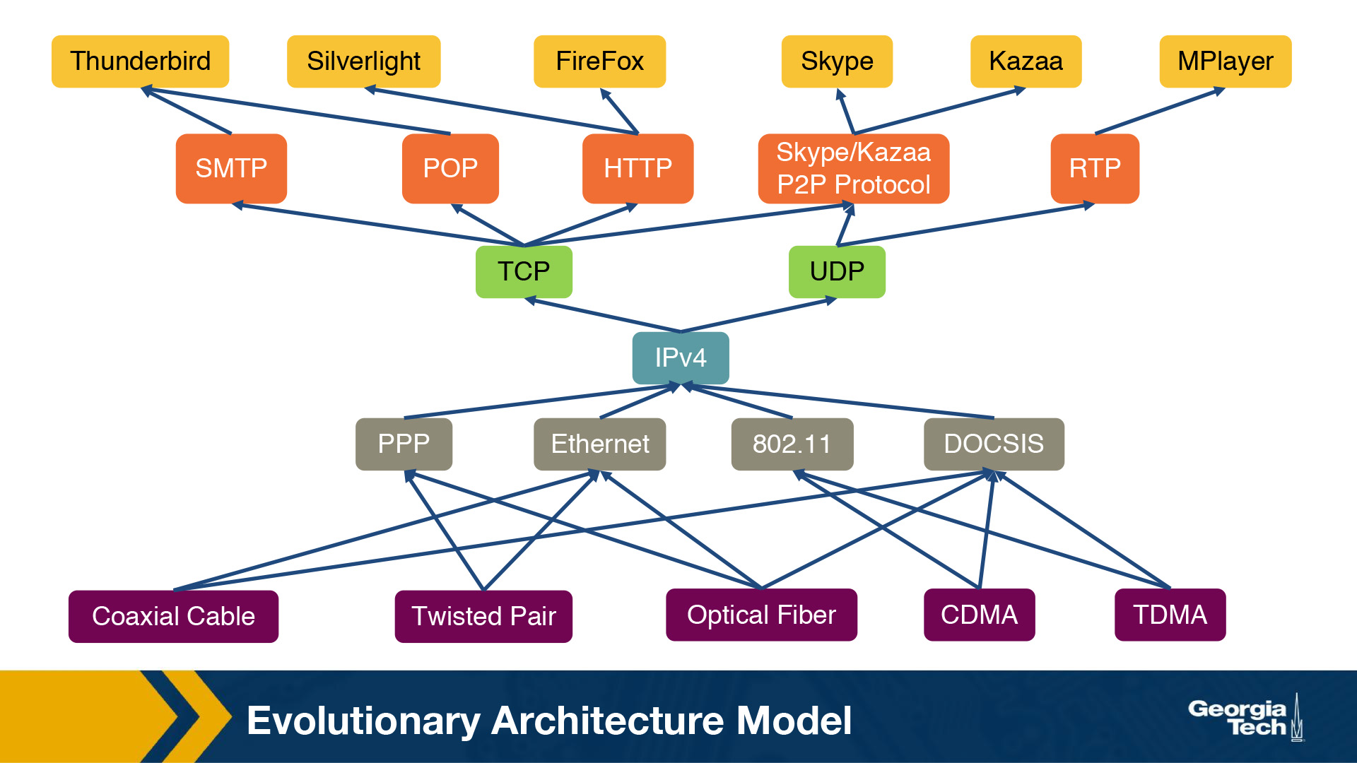
All roads lead to IP, and TCP/UDP. Researchers have actually done a lot of work to see why this is. They called it the evolutionary architecture model. They did a bunch of in depth quantifications of why/what the internet is and how they got there and drew some interesting conclusions.

In an ideal world where we could do it all over they came up with the following:

Finally, in terms of future and entirely new Internet architectures, the EvoArch model predicts that even if these brand-new architectures do not have the shape of an hourglass initially, they will probably do so as they evolve, which will lead to new ossified protocols. The model suggests that one way to proactively avoid these ossification effects that we now experience with TCP/IP is for a network architect to design the functionality of each layer so that the waist is wider, consisting of several protocols that offer largely non-overlapping but general services, so that they do not compete with each other.

Interconnecting Hosts and Networks

Talking about how to theoretically communicate between computers is important, but hardware actually makes the physical connections.

Those are:

Repeaters and Hubs

They operate on the physical layer (L1) as they receive and forward digital signals to connect different Ethernet segments. They provide connectivity between hosts that are directly connected (in the same network). The advantage is that they are simple and inexpensive devices, and they can be arranged in a hierarchy. Unfortunately, hosts that are connected through these devices belong to the same collision domain, meaning that they compete for access to the same link.

Bridges and Layer-2 Switches

These devices can enable communication between hosts that are not directly connected. They operate on the data link layer (L2) based on MAC addresses. They receive packets and forward them to the appropriate destination. A limitation is the finite bandwidth of the outputs. If the arrival rate of the traffic is higher than the capacity of the outputs, then packets are temporarily stored in buffers. But if the buffer space gets full, then this can lead to packet drops.

Routers and Layer-3 Switches

These are devices that operate on the network layer (L3).

Learning Bridges

A bridge is a piece of hardware that manages the connection between many devices, connected to the same piece of hardware.

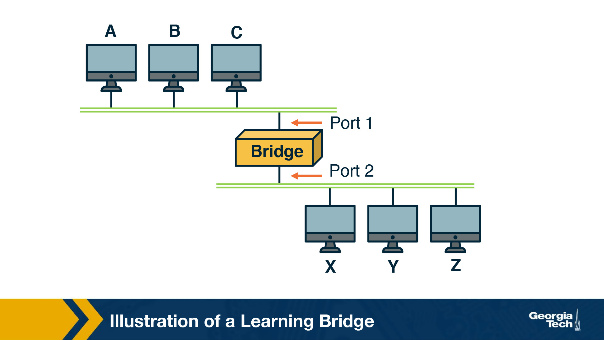
The bridge is able to understand what devices are on port 1, what devices are on port 2, and so on. This is like a home network switch. You can connect many devices to it, and it handles knowing where the data needs to end up.

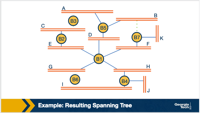
The Looping Problem

The problem with these bridges, is that you can create a loop.

if A connects to B which connects to C which connects to A, you’ve created a loop. This can result in never ending looping!

This is handled by running a spanning tree algorithm. The goal of the spanning tree algorithm is to identify which ports when used will eliminate any endless looping.

This works by operating in rounds, and then by removing bridges from the network until you only have one path to every node. This is accomplished by running in rounds the following process:

1. Every node sends:
   • Sender Node ID
   • Root ID as perceived by sender
   • Distance from root node
2. Each node selects the best configuration in order of
   • If root of the one configuration has a smaller ID
   • If roots have equal IDs choose one with smaller distance to the root
   • If they have the same distance, choose configuration with smallest sender ID
3. A node stops sending configuration messages over a link (port) when it receives a configuration message from a neighbor that is:
   • either closer to the root
   • has the same distance from the root, but it has a smaller ID.

We can see this process completed in the following images:

Then after tree spanning:

Lesson 2 - The Transport Layer (TCP)

This lesson is going to talk about the actual protocol responsible for transporting data from one location to another, TCP. The logical connection between two hosts is done in the transport layer.

The transport layer receives a message from the application layer and appends its own header on to it. This is known as a segment. The segment is then sent to the Network layer where it happily bounces through all the routers, bridges, and switches that might be on its path.

Transport Layer intro

Why do we need a transport layer? Why not just send messages directly from the application layer to the network layer? Because the network layer guarantees nothing. The transport layer guarantees delivery, and data integrity in a way that wouldn’t have been done otherwise.

As mentioned previously there are two main transport layer protocols User Datagram Protocol (UDP) and Transmission Control Protocol (TCP).

UDP just tries to quickly send data, and doesn’t do much else. As such it provides no guarantees and puts the responsibility on the application layer to do things like verify integrity and handle dropped messages.

TCP on the other hand does have these extra bells and whistles built in and thus it is much more reliable, if not a tad slower than UDP.

Multiplexing

Multiplexing is the ability for many hosts to use the same network simultaneously. Consider two computers browsing the internet at the same time, or better yet, a computer that is simultaneously browsing the internet and streaming music, it has two incoming data sources, and used in two different ways.

We need to be able to handle this complexity. The Transport layer uses ports to do this. Each application gets one port, and listens only to that port.

There is Connectionless and Connection Oriented multiplexing. One based on a constant connection, and one is not.

We have names for each direction of this multiplexing operation.

Demultiplexing - Delivering data to the appropriate socket.

Multiplexing - Taking data from all the sockets and putting it into the network layer.

Connectionless Multiplexing

Connectionless multiplexing is the simpler case. The transport layer has a segment which has the content, a source and source port, and a destination and a destination port. It receives the data from the source port, and makes its best effort at delivering to the destination port.

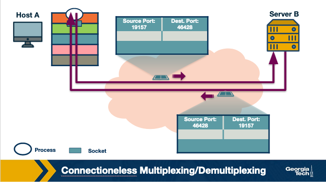
If the destination receives it, great, the network layer will route it to the correct port, and then the message will have been successfully delivered.

These are UDP sockets. It’s very direct, with no oversight as to what actually happens to the message.

Connection Oriented Multiplexing

Connection Oriented multiplexing brings in a lot more complexity.

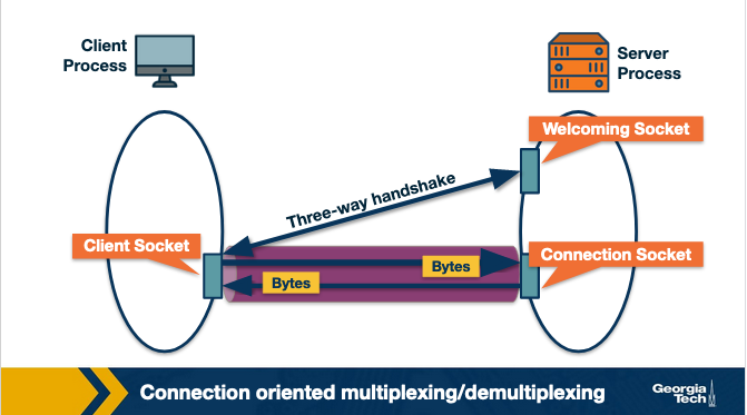
TCP requires going through a TCP server. The TCP server has a listener process that waits for incoming connection requests, and when it gets it handles setting everything up so that the destination is ready to receive the message.

Note: If a server has many clients contacting it on the same port, it’s not an issue because they have unique IP addresses (hopefully) and they can distinguish the difference between the two that way.

A word on UDP

UDP lacks reliability of TCP mainly because it doesn’t require establishing a connection.

That lack of reliability makes it better for the following reasons:

1. No congestion control - No process watches every packet to make sure it should be sent
2. No connection management - We don’t have to wait for a socket to be opened, so it just sends quickly

Both of these result in lower latency transmission, which is good for some things. Things like multiplayer video games, DNS servers, and other networking hosts, all like to use higher speed protocols.

This puts the onus on the developers on each end to ensure quality, and handle if errors occur, but when things are working well, then things are very speedy.

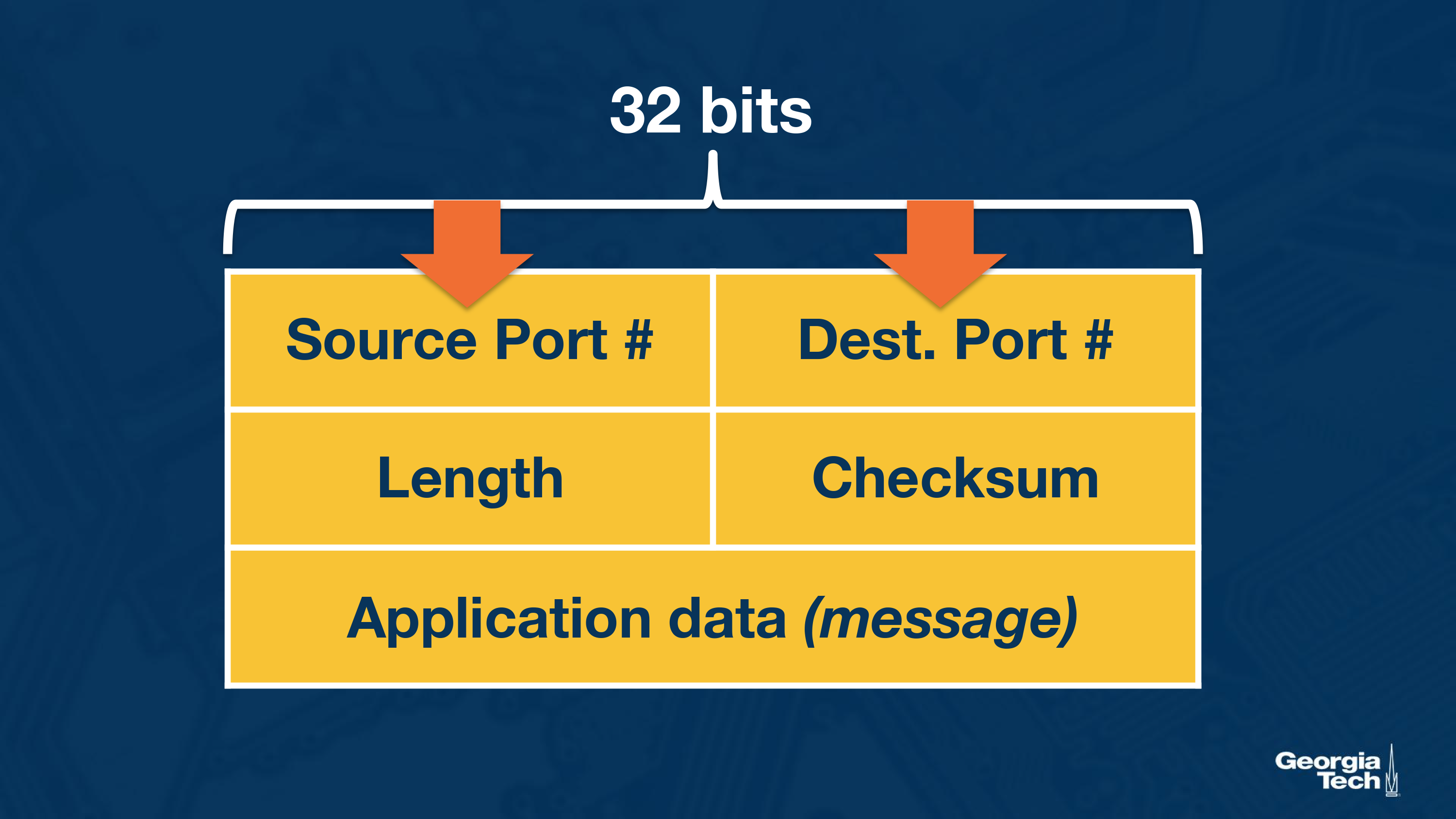
The one quality mechanism UDP provides is a checksum, so you can in fact check that the data that’s sent is what it was supposed to be. It creates a checksum by adding together the bits of the source port, destination port and the length of the packet. It then performs a ones complement. That is the checksum.

The receiver takes the source port, destination port, length of packet, and the checksum and adds them all together. Because the checksum is the ones complement, when they are added together it should end up as all ones.

TCP

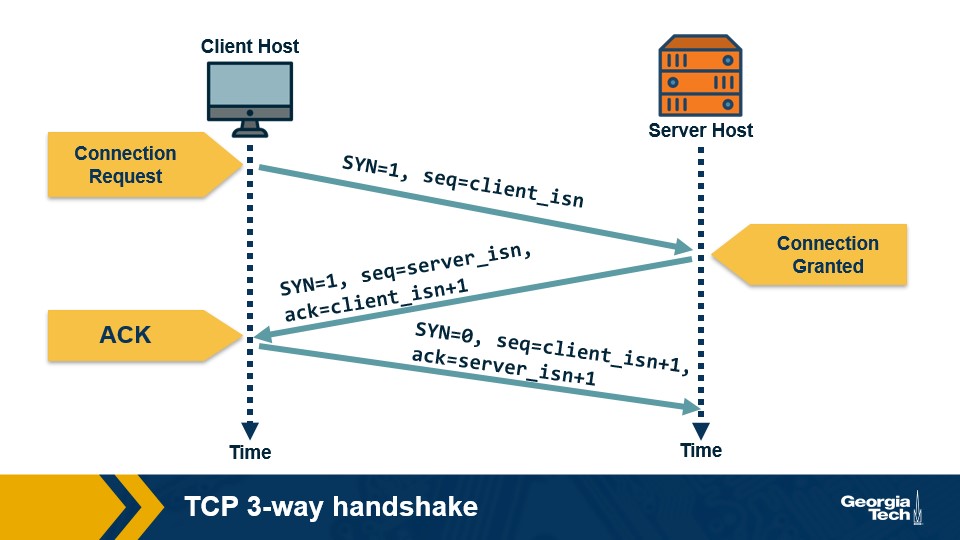
Three way handshake

Step 1: The TCP client sends a special segment (containing no data) with the SYN bit set to 1. The client also generates an initial sequence number (client_isn) and includes it in this special TCP SYN segment.

Step 2: The server, upon receiving this packet, allocates the required resources for the connection and sends back the special “connection-granted” segment which we call SYNACK segment. This packet has the SYN bit set to 1, the acknowledgement field of the TCP segment header set to client_isn+1, and a randomly chosen initial sequence number (server_isn) for the server.

Step 3: When the client receives the SYNACK segment, it also allocates buffer and resources for the connection and sends an acknowledgment with SYN bit set to 0.

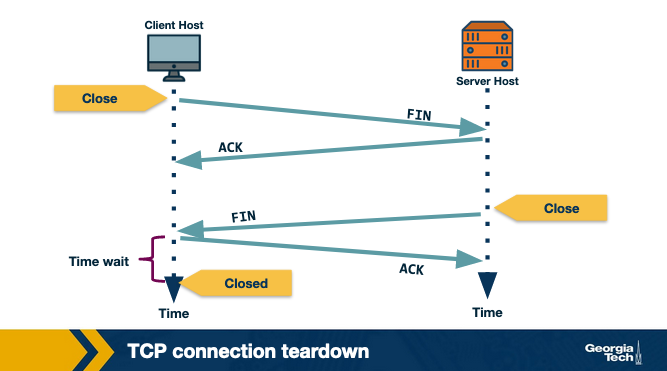
Connection tear down

Connection Teardown

Step 1: When the client wants to end the connection, it sends a segment with FIN bit set to 1 to the server.

Step 2: The server acknowledges that it has received the connection closing request and is now working on closing the connection.

Step 3: The server then sends a segment with FIN bit set to 1, indicating that connection is closed.

Step 4: The client sends an ACK for it to the server. It also waits for some time to resend this acknowledgment in case the first ACK segment is lost.

Reliable Transmission (TCP)

TCP guarantees all packets delivered in order. This is a very helpful reliability for developers to build on.

To do this the sender must know what the receiver successfully got. This is accomplished via ARQ (Automatic Repeat Request). If a sender doesn’t get a message that ARQ1 was received in a certain timeframe, then it will re-send it.

Stop and Wait ARQ

Guess how long it should take, if you don’t get a response, send it again. This can work but is tricky. If you send too much you’re retransmitting for no reason, and wait too long your connection is slow.

TCP uses Selective ACK which basically waits for the receiver to say hey I didn’t get this packet yet, and if it reaches a certain threshold like 3, then it will quickly resend that particular packet. This allows most of the time to be spent actively sending data, and the ability to recover from dropped packets.

This does require the ability to buffer packets until you have everything you need in order.

Transmission Control (TCP)

Deciding how much of a link bandwidth to use is a bit complicated. If you send too much for the receiver that could be an issue, or maybe the network can’t handle it, or any other amount of things that could go wrong.

So TCP implements a couple things to help that.

Flow Control

Flow control is where TCP tries to identify the receiver’s buffer that it is receiving data with, and tries to match the sender window size to that. Every ACK message includes a rwnd value which says how much buffer space is available.

The sender uses this value to ensure it never sends more bytes than is available in the receiver buffer.

If this value hits zero it would stop, but TCP instead sends packets of 1 byte until it gets a response with a rwnd greater than zero.

Congestion Control

Congestion control is making sure we don’t overload any of the links on the way from one host to another.

Good congestion control is:

• Efficient - use most of the network
• Fair - everyone gets equal amounts
• Low delay - Low delay is good for things that need to have small lag like video conferences
• Fast convergence - everyone gets their bandwidth quickly

Network Assisted

Network assisted congestion control relies on pieces of the network sending feedback about what’s happening. This could fail when the network is heavily congested though, kind of rendering it useless.

End to End

End to end congestion control gets nothing from the network and instead infers congestion from the hosts. This supports the general principle of making the complexity be at the ends of the networks.

This is mostly done via packet delay (how long did it take to get here) and packet loss (how many times do I need to resend). With these two things you have a rough understanding of network performance at any given moment.

It employs a congestion window, a number indicating roughly how much space is left in the network. This increases until congestion is detected, and then the window is made smaller to reduce congestion.

Ultimately the max size of a TCP packet is the minimum of the receiver buffer and the congestion window.

There are many different methods of increasing congestion window size:

• Additive
• Multiplicative
• TCP Reno
• AIMD

Many of these employ “Slow start” where they start at a low-ish speed and ramp up. This protects from overwhelming the network right at the start. With timeouts or dropped connections being common you can see why this would be useful.

TCP isn’t always fair, but using some of these congestion methods will do a pretty good job of it.

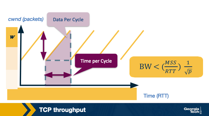
TCP Throughput

TCP Throughput looks like a sawtooth because of these congestion control mechanisms.

It gets up to the limit, then drops off, then gets up to the limit then drops off.

Lesson 3 - Intradomain Routing (The Network Layer)

This session focuses on the act of routing on the network layer in a single domain. Ideally we understand what it takes for two hosts to share data by the end of this.

We’ll talk about:

• Intradomain Routing Algorithms
  • Link state
  • Distance vector
• Intradomain Protocols
  • Open Shortest Path First (OSPF)
  • Routing Information Protocol (RIP)

Routing

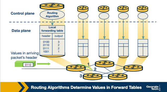
Given two hosts that share the same default router (first-hop router) we know that one host will send a packet to the default router, but what happens next?

In a network with many routers, whenever a router receives a packet, it must consult the forwarding table it maintains, and send the packet to the next router in line. This is referred to as forwarding and is not necessarily the same as routing.

Routing is the act of determining the best path to be traveled from one location to another. Intradomain routing is what we will focus on and it is what happens when both hosts are in the same administrative domain.

Interior Gateway Protocols (IGP) are what handle this type of routing. The two major types we’ll cover are link-state and distance-vector routing algorithms. They are graph theory algorithms with edges and nodes.

Link State Routing

Surprise, Dijkstra’s algorithm is here again.

In link state, all link costs are known and the network topology is also fully known.

From the lecture directly.

Let’s introduce some basic terminology. By u, we represent our source node. By v, we represent every other node in the network. By D(v), we represent the cost of the current least cost path from u to v. By p(v), we represent the previous node along the current least cost path from u to v. By c(u,v), we represent the cost from u to directly attached neighbor v. By N’, we represent the subset of nodes along the current least-cost path from u to v.

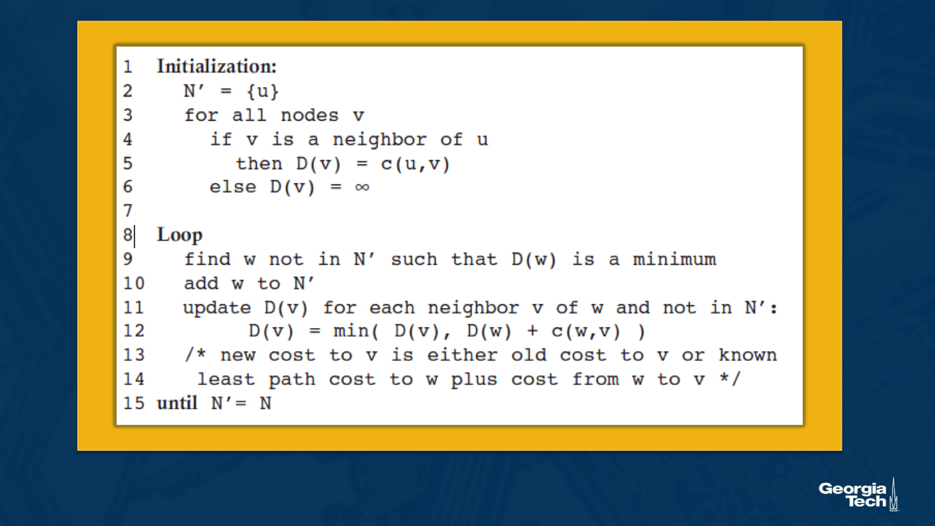
Basically we initialize with either:

• Known cost because it’s a link directly connected to the node we’re initializing
• Infinity cost, because we know it will be less than that but we have something to compare against

Then we continue looping through the network, looking for a path with lower costs than our current cost, until we don’t find one. This is a fun application of Dijkstra’s algorithm, where each router essentially computes Dijkstra’s algorithm from itself to all other routers in the network.

This is a pretty costly algorithm at O(n^2) complexity. It also requires that you know everything about the network which is probably why this is intradomain and not interdomain.

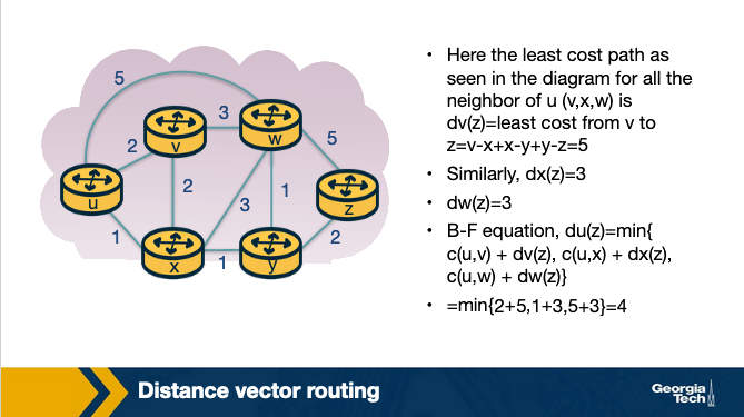
Distance Vector Routing

The DV algorithm is iterative, asynchronous, and distributed.

DV is based on the Bellman Ford algorithm. Every node maintains a distance vector to all of the other nodes, and it occasionally shares that information. When a node receives a new distance vector they use it to update their own vector.

The Bellman Ford (BF) equation is the heart of each update: Dx(y) = minv{c(x,v) + Dv(y)}

See the pseudocode below:

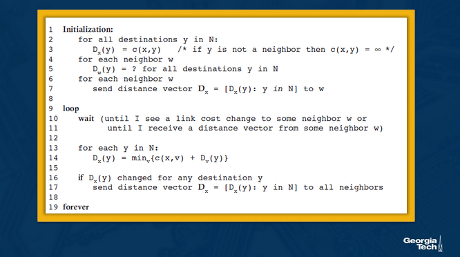
So essentially, continuously the nodes maintain a list of costs for routes to certain nodes, and these costs are updated whenever nodes send their costs. So instead of every node needing to know every cost, it allows the nodes to only know and focus on the costs of its immediate neighbors, and then relies on other nodes sending its current list of costs occasionally.

This is different from Link State routing because it is distributed, but they are all still computing the most efficient path through the tree.

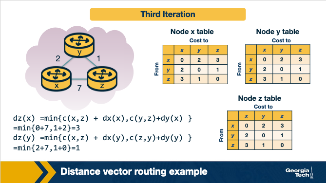
A simple example

initialization

Pitfalls of DV

What if the link cost changes? In some cases this is handled quickly, and in other cases it can lead to a “count-to-infinity” problem.

Say a link cost decreases:

1. At time t0, y detects that cost to x has changed from 4 to 1, so it updates its distance vector and sends it to its neighbors.
2. At time t1, z receives the update from y. Now z thinks it can reach x through y with a cost of 2, so it sends its new distance vector to its neighbors.
3. At time t2, y receives the update from z. Y does not change its distance vector, so it does not send any update.

The update is fully propagated pretty quickly.

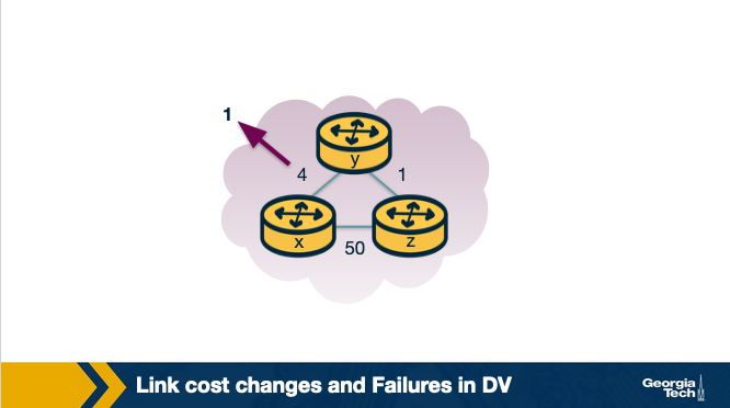
Say a link cost increases:

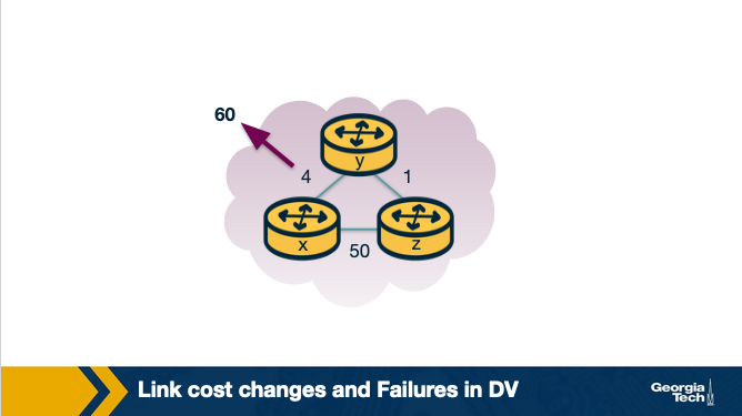
1. At t0, y detects that the cost has changed, and now it will update its distance vector thinking that it can still reach x through z with a total cost of 5+1=6.
2. At t1, we have a routing loop where z thinks it can reach x through y, and y thinks it can reach x through z. This will cause the packets to be bouncing back and forth between y and z until their tables change.
3. Nodes z and y keep updating each other about their new cost to reach x. For example, y computes its new cost to be 6 and then informs z. Then z computes its new cost to be 7, and then informs y, and so on.

The key here is that Node Z, is saying Hey I can definitely reach X, and the cost as Z knows it, is 5. So Node Y says sweet, if I go through Node Z, it’s the cost of our link (1) + the cost of Z > X, but the cost of Z > X isn’t actually 5 anymore, it’s 50.

So they have to iterate until the cost is greater than 50, at which point it will use the real path.

The reason that we can’t directly say, “hey no the link cost increased by a ton your table is wrong” is because we don’t know the structure of the network. All we know is X > Y costs a certain value, with no understanding of which links do that.

So instead we have to keep iterating through until the costs are actually updated. This can create a lot of packet bouncing.

This is solved by something called poison reverse where a node says a cost is infinity if it isn’t the cheapest path to a certain node. This only works for 2 nodes.

Routing Information Protocol (RIP)

RIP is based on Distance Vectors, but instead of maintaining vectors of distances, they instead maintain entire routing tables with one row for each subnet.

Open Shortest Path First

OSPF is a routing protocol that uses link-state to find the best path between source and destination routers. It was created after RIP by ISPs with extra things like authentication messages, multiple same-cost paths, and support for hierarchical routing within a single domain.

OSPF will have one AS (Autonomous System) as the backbone, and routes to other OSPF AS on the network. To go from one Area to another, they must move through the backbone router.

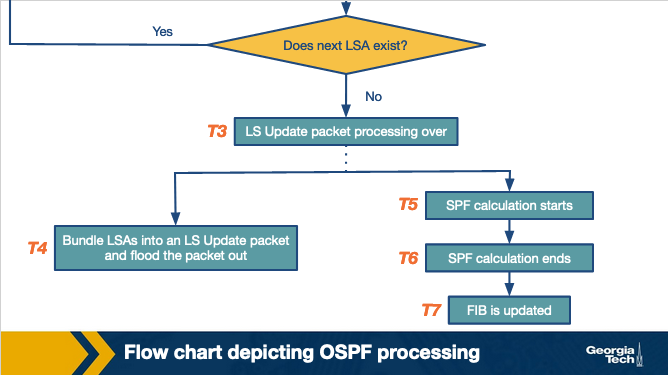
There’s a lot more in the notes but tbh they’re pretty complicated! It seems that these routers in the send Link State advertisements which communicates the routers local topology. This results in a complete network map, that updates when the network updates.

These LSAs are processed as so:

Hot Potato Routing

Sometimes you have to leave your local network, and enter into interdomain routing.

To do this usually you have to find an egress point and the process of finding that egress point is an intradomain routing problem.

Generally hot potato routing is referring to finding the closest/least costly egress point in a given network. The hot potato part of it is that there are many egress points and which one is chosen is not always clear. This routing method of finding the shortest path does make things consistent instead of sometimes going to egress A and sometimes going to egress B.

Lesson 4 - Interdomain Routing and AS Relationships

Lesson 3 focused on intradomain routing, but what about when we need to leave our domain?

The internet is an ecosystem of thousands if not millions of networks operated independently, but still connected to each other. This lesson we’ll learn about BGP.

The Internet

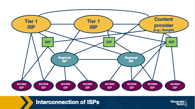
The internet started very hierarchical but has been flattening as more IXPs and CDNs have been added.

Each of the types of infrastructure above can be an Autonomous System (AS) which is a group of routers who are under the same authority. I think like, my house technically is an AS that I manage, but not sure about that.

Routing between AS’s relies on Border Gateway Protocol (BGP) to exchange information with each other.

AS Ecosystem

There’s two main interactions between AS’s.

• Provider-Customer - Like me paying my ISP for internet
• Peer - One ISP routing to another ISP because they need their network to get to location x. This requires traffic levels to be pretty similar so that one party isn’t gaining more than the other.

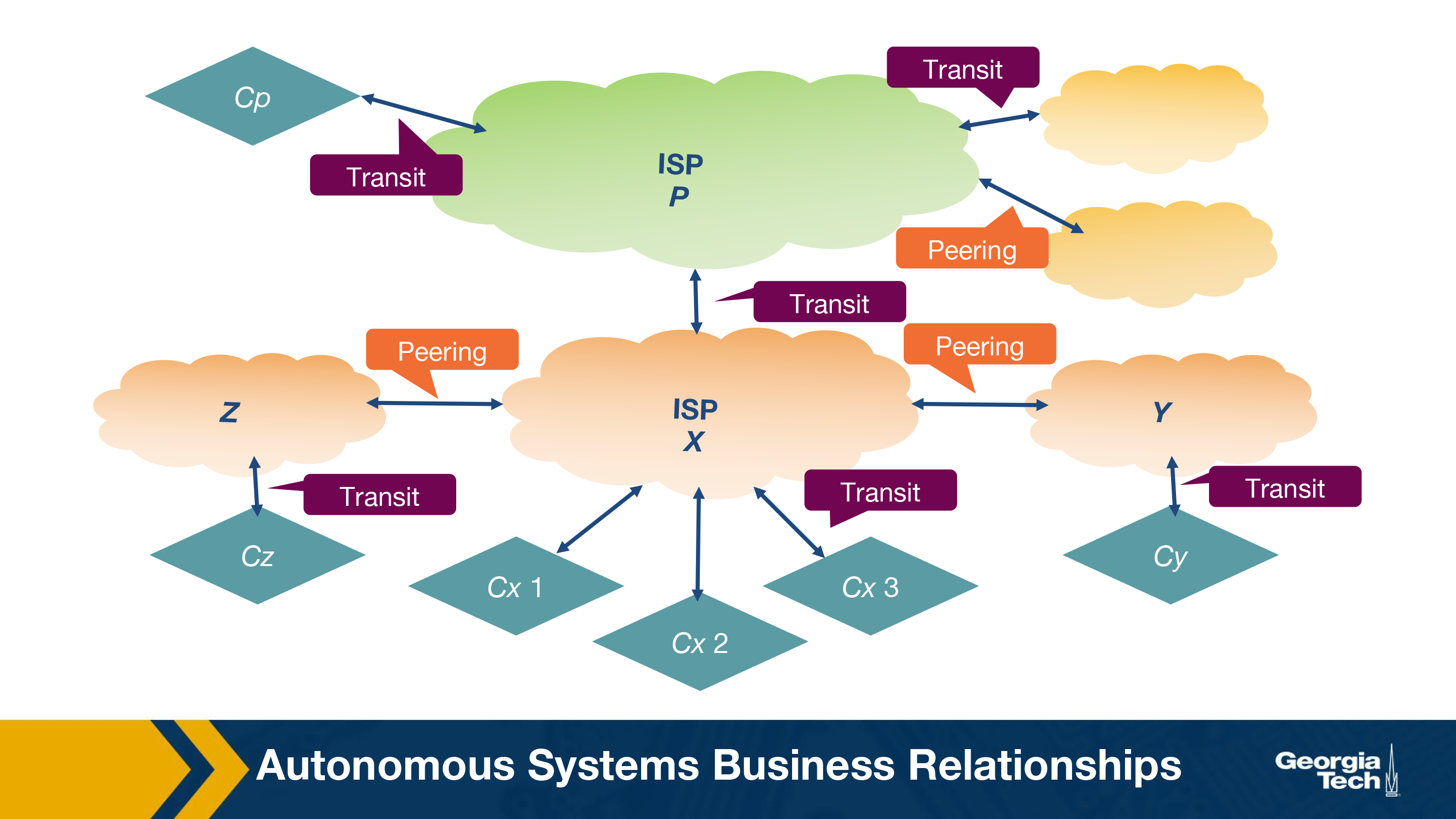
See how green cloud ISP can’t peer with orange cloud ISPs, because it’s too large. But all the orange cloud ISPs are peer relationships because they’re similarly sized.

Providers can charge fixed rate or based on usage, totally up to them.

Internet Business

Importing and Exporting routes is the heart of BGP. Deciding which import/exports to operate and make available is a technical and business decision.

Exporting Routes

Export routes come from:

• Routes from customers
• Routes from providers
• Routes from peers

Which of these are chosen to advertise to other AS’s is a business decision.

Importing Routes

Again, they’re picky based on which routes are going to bring the most value to the business.

Usually it’s this order:

1. An AS wants to ensure that routes toward its customers do not traverse other ASes, unnecessarily generating costs.
2. An AS uses routes learned from peers since these are usually “free” (under the peering agreement).
3. An AS resorts to importing routes learned from providers only when necessary for connectivity since these will add to costs.

Border Gateway Protocol (BGP)

BGP Design Goals

• Scalability - The internet will never stop growing, try to handle it
• Express routing policies (ERP) - Allows ASes to make routing decisions and do it privately
• Allow cooperation among ASes - Allows ASes to make their own decision and let business drive the connections
• Security - This was added on as it was found to be necessary

BGP Basics

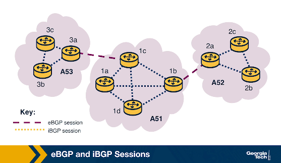
BGP Peers send messages over BGP Sessions over a semi-permanent TCP port connection. A session is initiated from one router to another with an OPEN message which is then followed by sharing routing tables.

eBGP is an external BGP session, between two ASes. iBGP is an internal BGP session, in a singular AS.

Once the session is started they use:

• UPDATE - if any updates are made to the Route table, share it
• KEEPALIVE - Keeps session going, no changes

BGP relies on prefix reachability, a list of IP addresses that prefix all the destinations. This is how the export and import routes are communicated.

Other parameters:

Path Attributes are also shared with other providers with parameters like:

• ASPATH - Contains Autonomous System Number and helps choose between multiple routes and stops loops
• NEXT HOP - Provides the next router’s IP address so that other routers can store in their forwarding table the best path

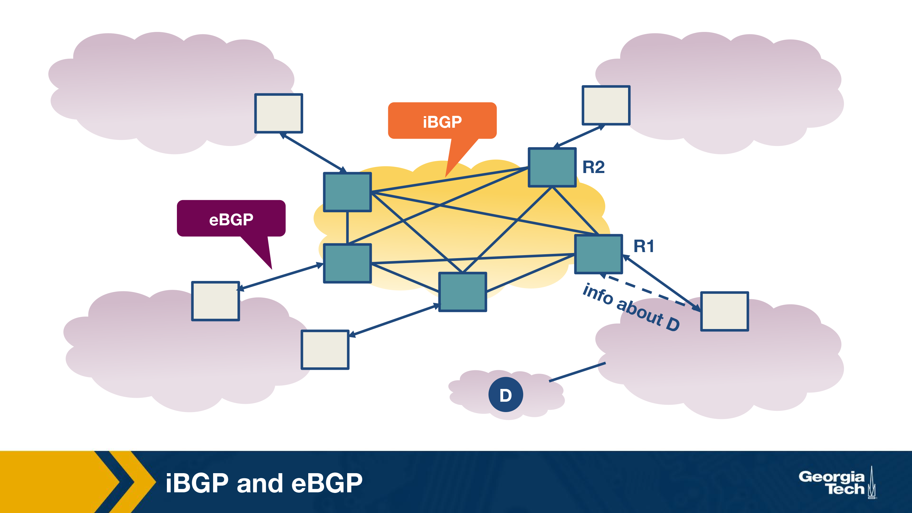
iBGP vs eBGP

iBGP is meant for sharing paths of how to get out of an AS, it’s not an IGP that gives intradomain networking, but instead a way of telling nodes inside of AS how they can communicate with external ASes.

eBGP is the method of communicating between ASes the available external routes.

BGP Router Process

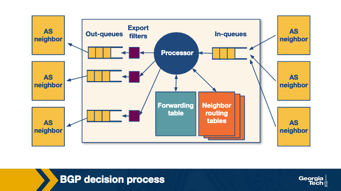
When a router receives a new list of policies it takes them all in, and then has a decision making process to determine the best routes for it to use.

The operator of this router can determine what is important to them (usually cost related) and make decisions based on that. Here’s an example decision process.

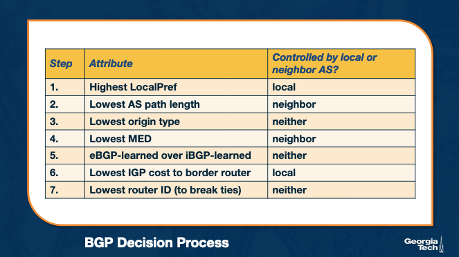
Important decision makers are:

LocalPref - Decided by operating AS, things like choose the cheaper route (customers first, then peers, etc) MED - Determined by the neighboring AS, determine which link they would prefer you to use

BGP Issues

Two main things:

• Misconfiguration - Improper configuration can bring networks down for a lot of reasons
  • Can be reduced by limiting size of tables and number of changes
• Scalability - Large routing tables are problematic.

A lot of work went into reducing routing table sizes. They will do things like use default routing, route aggregation, and something called flap damping. Flap damping is a technique that limits the number of updates to a given prefix over time. If it goes over a certain limit, it will silence that prefix’s updates until a set time has passed.

This is configurable by domain, allowing you to choose when and where you will accept a lot of updates and when you won’t.

Peering at IXPs

ASes peer with each other, where do they do that? One place is an Internet Exchange Point (IXP). They are purpose built infrastructure to facilitate peering.

Internet Exchange Points (IXPs) are critical physical infrastructures where Autonomous Systems (ASes) can directly interconnect and exchange traffic. These facilities are typically housed in secure, well-powered data centers and consist of robust switch fabrics to ensure reliability and fault tolerance. ASes participating in IXPs must have a public ASN, a BGP-capable router, and agree to the IXP’s terms. Once connected, ASes can publicly peer and exchange traffic settlement-free, paying only for connection and port usage, not traffic volume. This makes IXPs more cost-effective and efficient than traditional third-party traffic routing.

IXPs have grown in popularity due to their ability to handle massive volumes of traffic and play a crucial role in improving network performance and reducing costs by keeping local traffic local. They also offer defensive benefits, such as DDoS mitigation, since they observe a large portion of Internet traffic and can help stop malicious activity before it reaches the intended target. Furthermore, IXPs provide a rich environment for research and innovation, particularly in areas like security and Software Defined Networking (SDN), and are evolving into hubs of technology development beyond just traffic exchange.

In addition to public and private peering services, IXPs offer a wide range of features such as route servers, SLAs, remote peering via resellers, mobile network peering, and DDoS blackholing. Some IXPs also provide free value-added services like DNS root servers and time distribution. These offerings, along with the ability to form fast and scalable peering agreements, have made IXPs essential infrastructure for global Internet connectivity, performance, and resilience.

Route Servers

IXPs use route servers to handle the large number of ASes that they service.

In summary, a Route Server (RS) does the following:

• It collects and shares routing information from its peers or participants of the IXP that connect to the RS.
• It executes its own BGP decision process and re-advertises the resulting information (e.g., best route selection) to all RS’s peer routers.

It’s basically offloading all the configuration work from the AS to the IXP operator. It’s what allows people like me to buy a domain and get reliable routing from anywhere in the world to it.

Lesson 5 and 6 - Router Design and Algorithms

Routers are what do the heavy lifting for actually moving data from one point to another. The prior lessons established many pieces and parts of that puzzle.

In short, a router needs to be able to receive an incoming packet on an input link, read its destination, and then send it to the correct output link. Simple in theory, difficult in practice, and more importantly, at scale. Then add on top of just forwarding requirements things like security requirements, quality of service, and other more advanced things, the job becomes difficult.

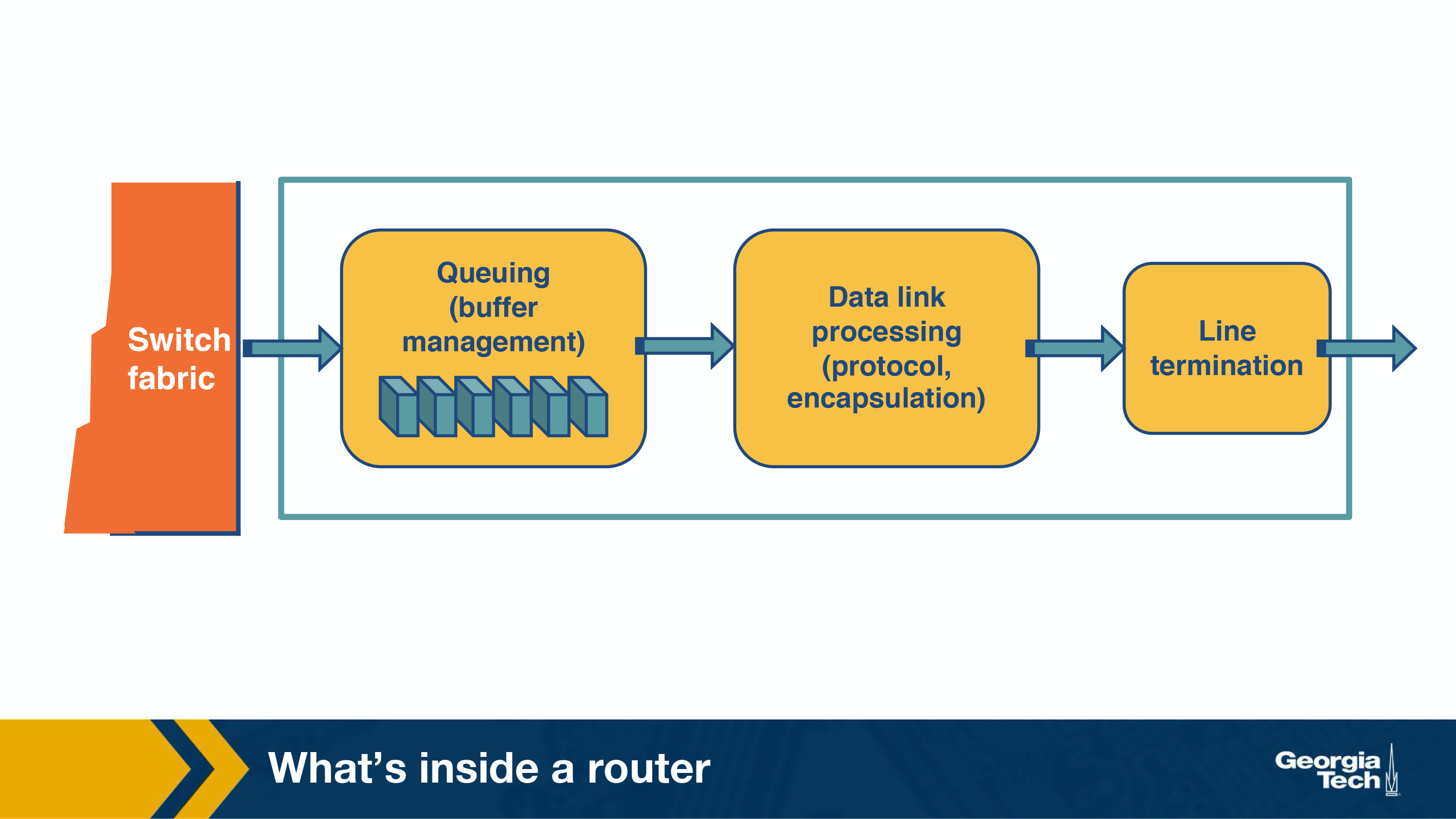
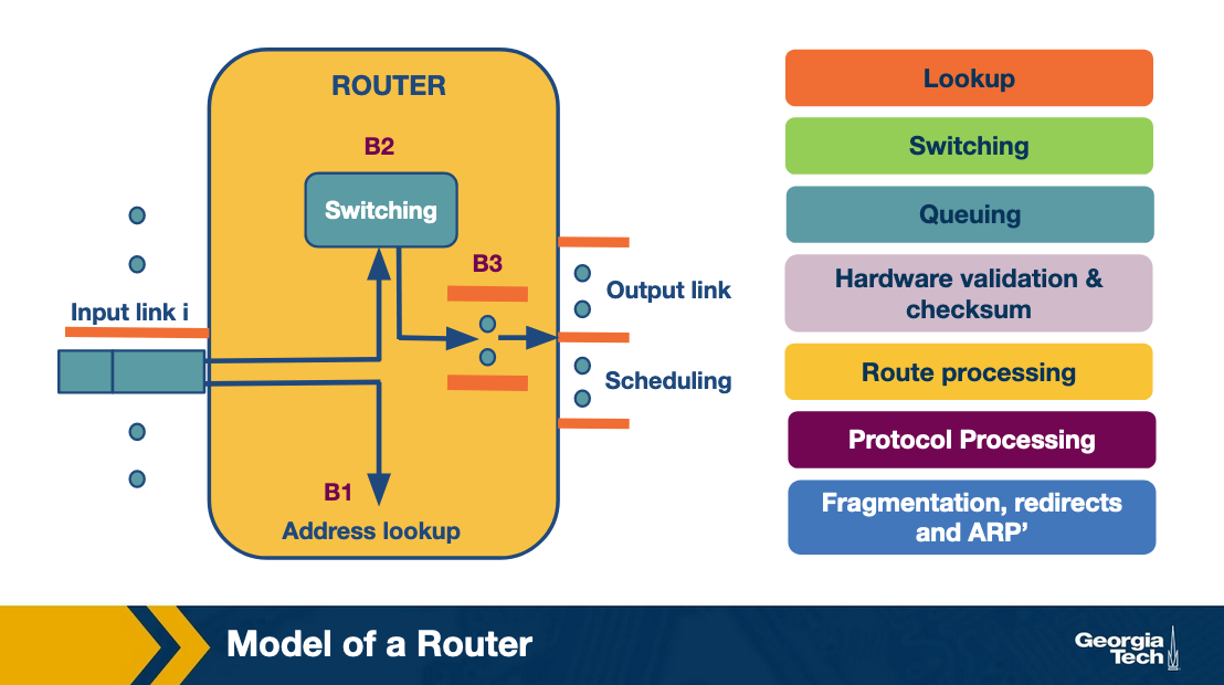
Router Components

The main job of a router is to implement the forwarding plane functions and the control plane functions.

Forwarding (Switching) function

The action of transferring a packet from an incoming link, to an outbound link. This should be very fast, on the scale of a few nanoseconds. I believe this is what a nice simple 5 port network switch is, and that’s all it is.

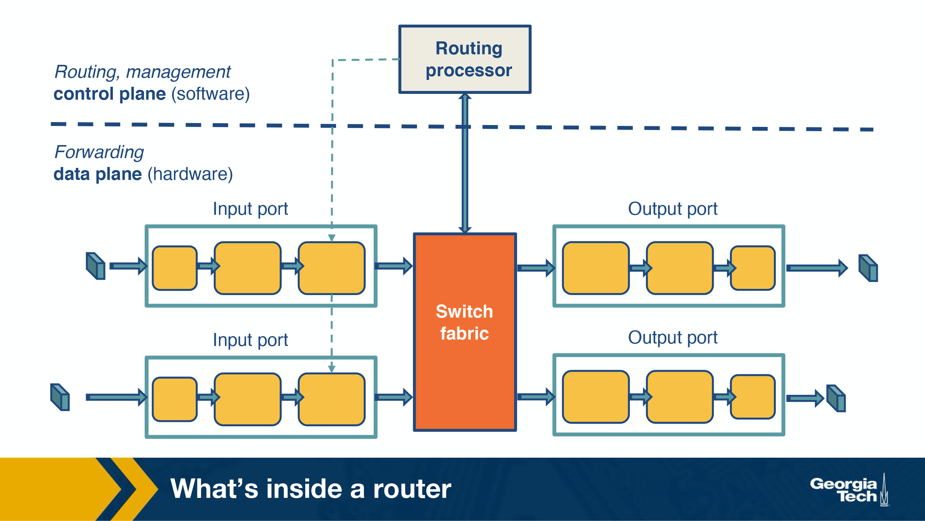
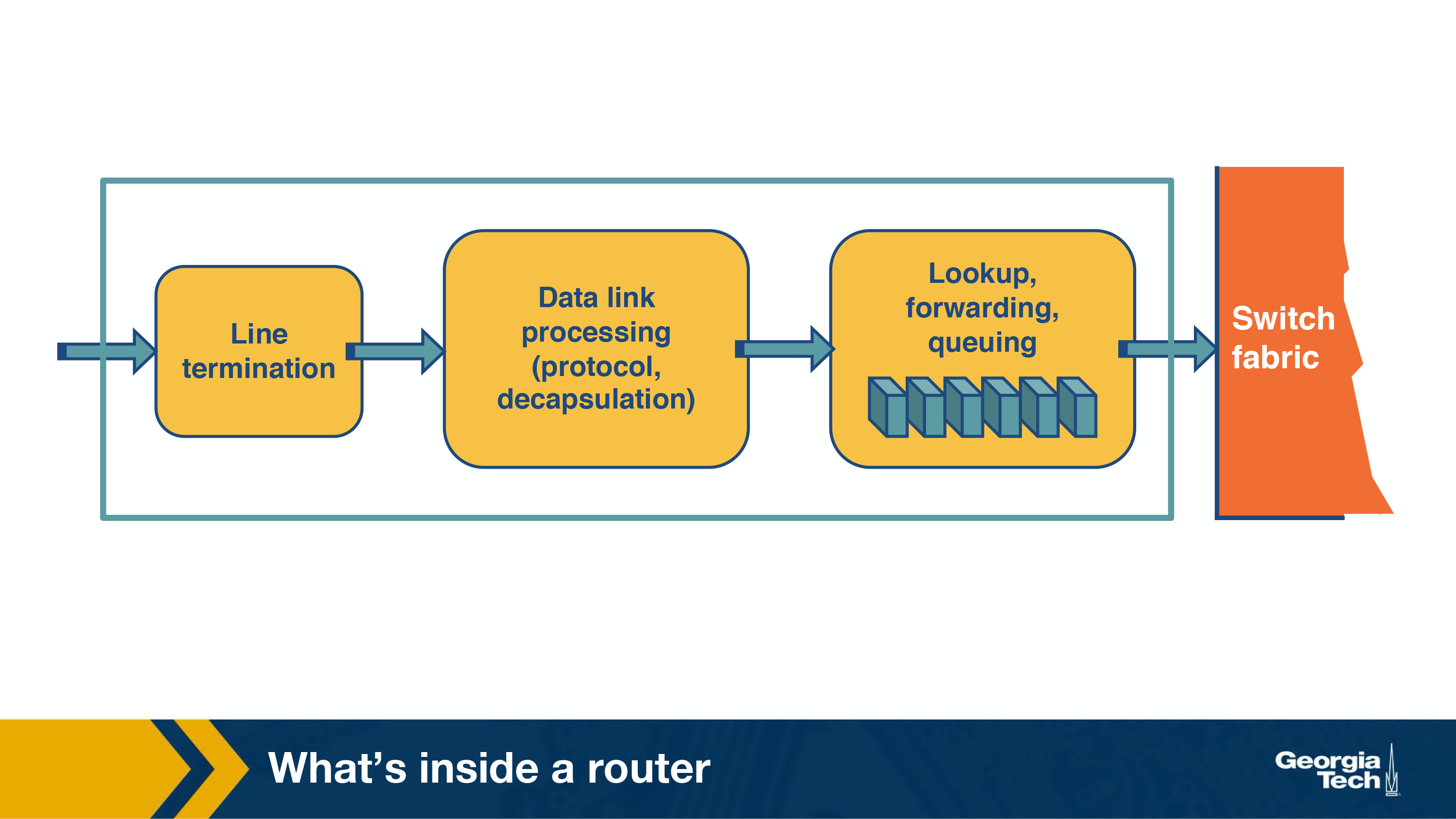
Input Ports

Input ports do the following:

1. Physically terminate the link
2. Processes datalink (decapsulating)
3. Performs lookup function, consulting forwarding table to determine where it should go

Switching Fabric*

This actually moves the packet from the input port, to the output port, using the results from the input port that tells where the packet needs to go.

Three types of switching fabrics:

• Memory
• Bus
• Crossbar

Output ports

All this does is receive the data from the switching fabric and send it. Specifically:

1. Queue the packets for transfer
2. Encapsulate the packets
3. Send them over the physical output port

Control Plane function

The control plane refers to:

• Implementing routing protocols (like the ones from earlier sessions)
• Maintaining routing tables
• Computing the forwarding table

All of these functions are written software in the routing processor, or in the case of an SDN, could be implemented by a remote router.

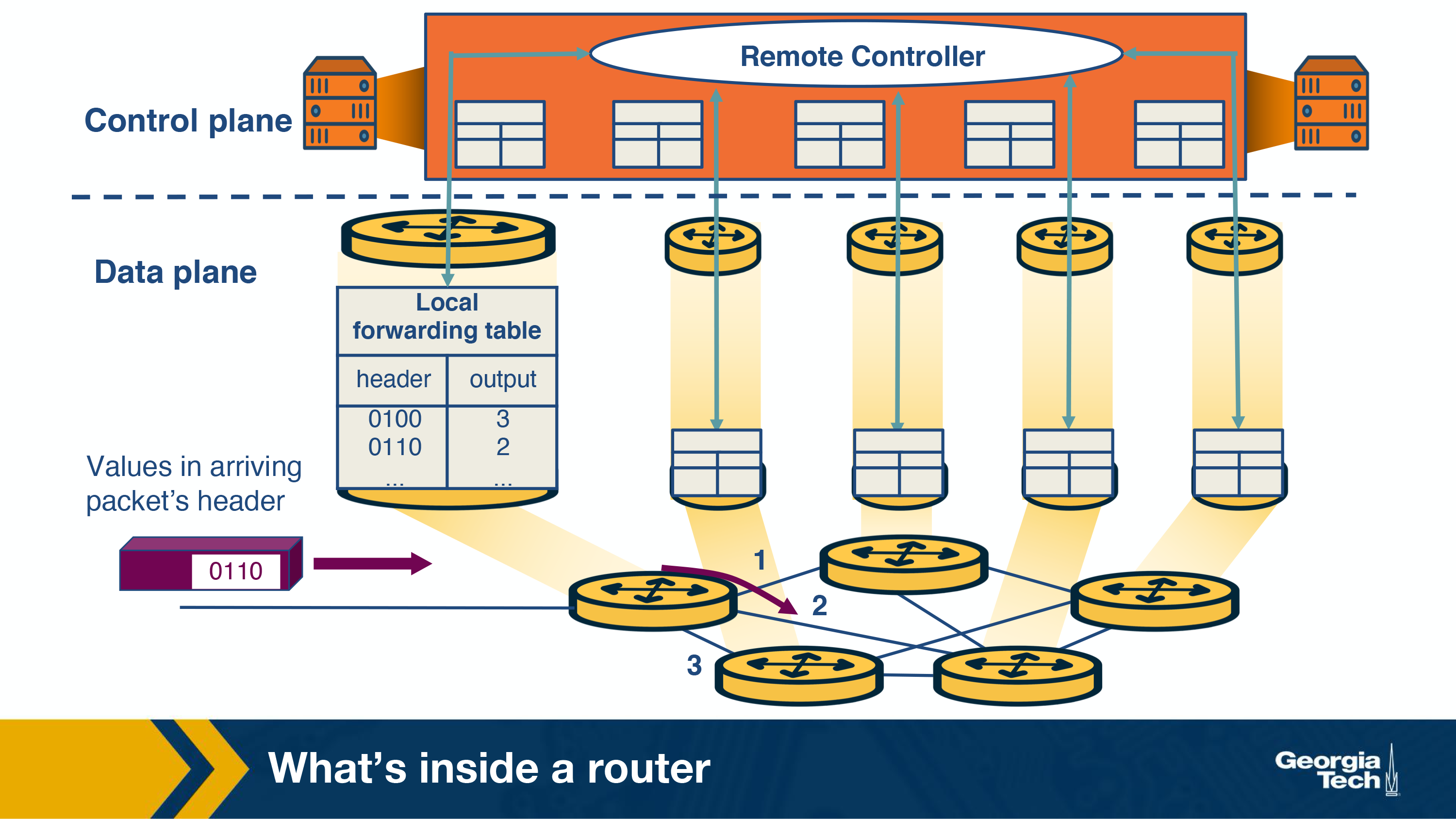
Router Architecture

Model of a router:

Using the image as a guide we can walk through the path that common tasks take. First we lookup the destination of an incoming packet.

1. Lookup
   1. Packet arrives at input link
   2. Lookup output link in forwarding table (Forwarding Information Base FIB)
   3. Resolve any ambiguities
      • Longest Prefix matching
      • Packet classification
2. Switching
   • After lookup is completed the packet is switched, from input link to output link. Modern routers use crossbar switches for this task.
   • Some complications occur when many inputs want to send to the same output
3. Queuing

   • Using various queuing logics, if an output port is congested, each packet enters the queue to wait its turn to use the hardware.

   • Types of queues used:

     • First In First Out (FIFO)
     • Weighted Fair Queuing
4. Header Validation and Checksum
   • Check version number, validate checksum, decrement ttl
5. Route processing
   • Build route using protocols like RIP, OSPF, and BGP
6. Protocol Processing (Including:)
   • Simple Network Management Protocol (SNMP) - Counters for remote inspection
   • TCP/UDP for remote communication
   • Internet Control Message Protocol (ICMP) for sending error messages (eg: TTL is exceeded)

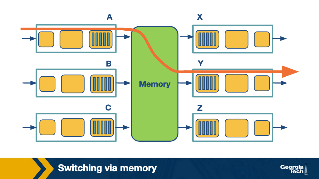
Switching Fabric

The switching fabric is where most of the logic is implemented in a router, forwarding packets from source to destination.

There are several ways to accomplish this.

Switching via memory

Physical I/O ports operate as I/O devices in an operating system.

1. Input port receives packet
2. Send interrupt to routing processor
3. Packet written to memory
4. Processor looks at header to get destination address
5. Lookup output port from forwarding table
6. Copy from memory into output ports buffer

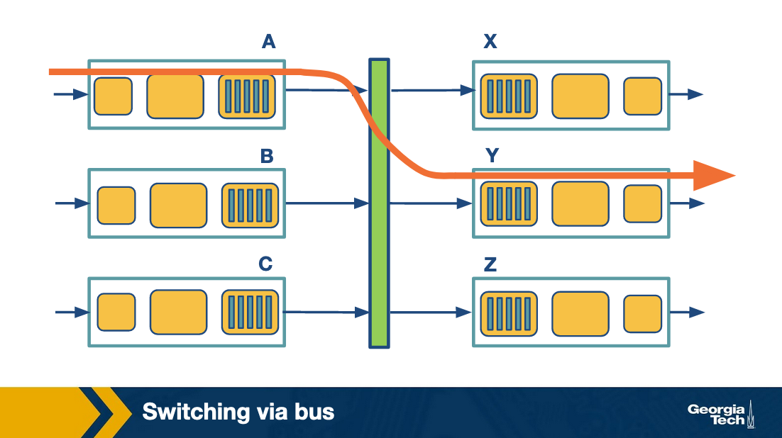
Switching via bus

Bus based switching doesn’t require a processor.

1. Input port receives packet
2. Input port marks which destination port it should be for with an internal header
3. Send it to the bus where all output ports receive the packet
   • Only the port it’s supposed to go to accepts it

This design is limited by the speed of the bus as only one packet can traverse it at a time.

Switching via interconnection network

A crossbar switch is an interconnection network that connects N inputs to N outputs using 2N buses.

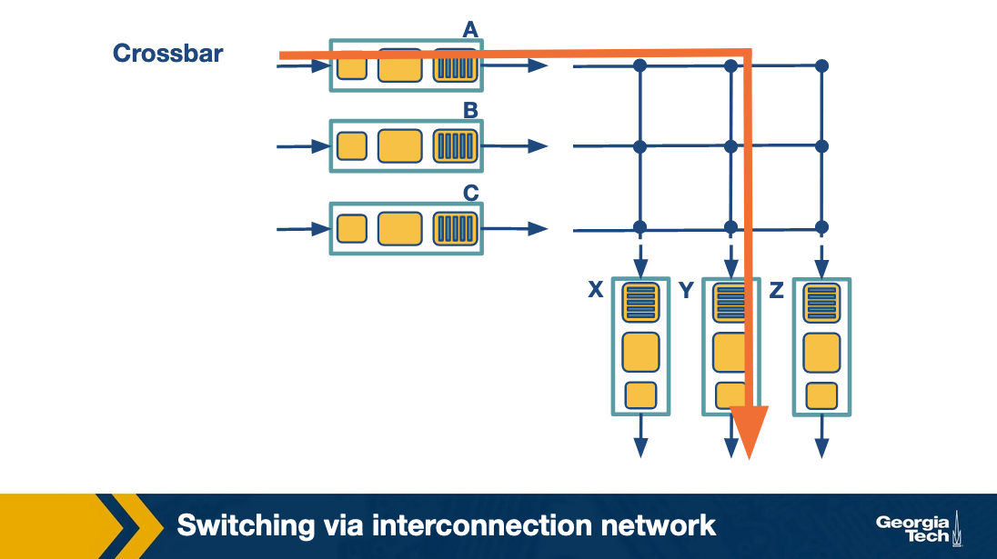
This allows many packets at once to traverse the switching fabric, as long as they have different input and output ports. This is done by giving the switching fabric control of the buses, and closing the connections to make the links only when there is a packet that needs to make that journey.

Router Challenges

There are a couple fundamental challenges to overcome for routers at scale.

1. Bandwidth and Internet population scaling
   • Rapidly increasing number of devices (endpoints)
   • Rapidly increasing volume of data
   • New types of links like optical links (fiber) which increase transfer but increase complexity
2. Services at high speeds

Common bottlenecks

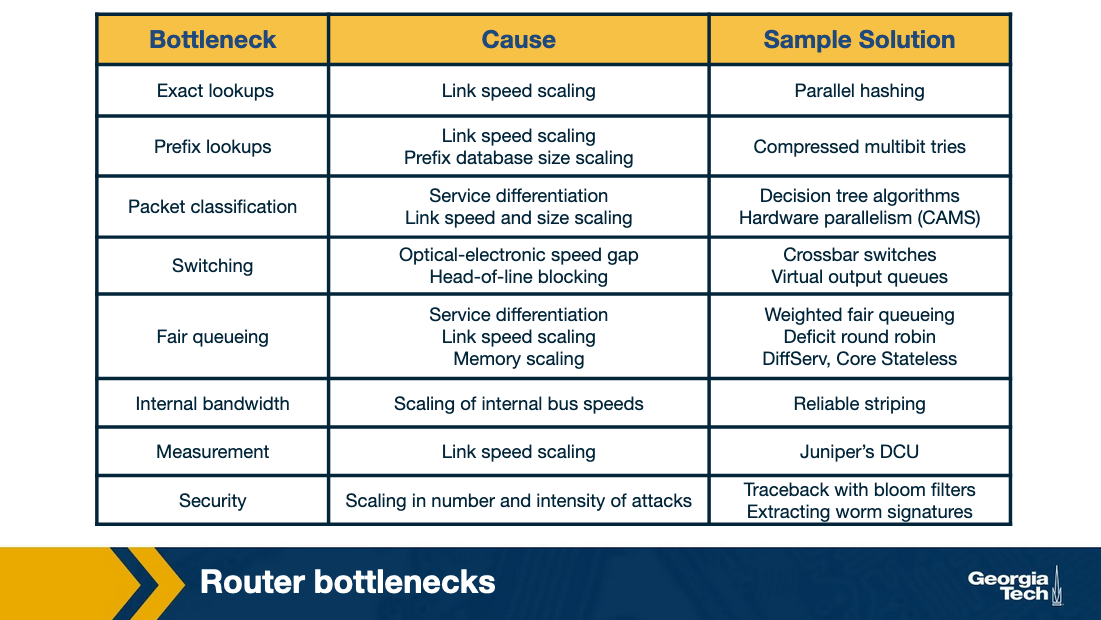
A little bit more detail:

Longest prefix matching - Due to the ever increasing number of devices on the internet, it’s impossible to hold a table for all of them. So instead devices are grouped into prefixes. But then you need good algorithms to deal with the prefixes.

Service differentiation - If you want to be able to provide priority to some packets and not to others, you need more complex logic to handle that. At scale.

Switching Limitations - At high speeds, the hardware can become a problem, causing bottlenecks at the I/O ports or even on the switching hardware.

Bottlenecks about services - Providing a reliable, fast, secure service that is guaranteed is difficult. Entire companies are built around doing this so that others don’t have to.

Prefix matching

Prefixing is a way to group endpoints together to make lookup tables less large.

Prefix Notation:

There are several ways to notate prefixes.

1. Dot decimal
   • 16 bit (132.234) becomes binary of 1000010011101010
2. Slash notation
   • A/L, A=Address, L=Length
   • 132.234.0.0/16
3. Masking
   • 123.234.0.0/16 is written as 123.234.0.0 with a mask 255.255.0.0
   • The mask 255.255.0.0 denotes that only the first 16 bits are important.

This prefixing helped, because we were running out of IP addresses, quickly. But it introduced the issue of longest matching prefix lookup.

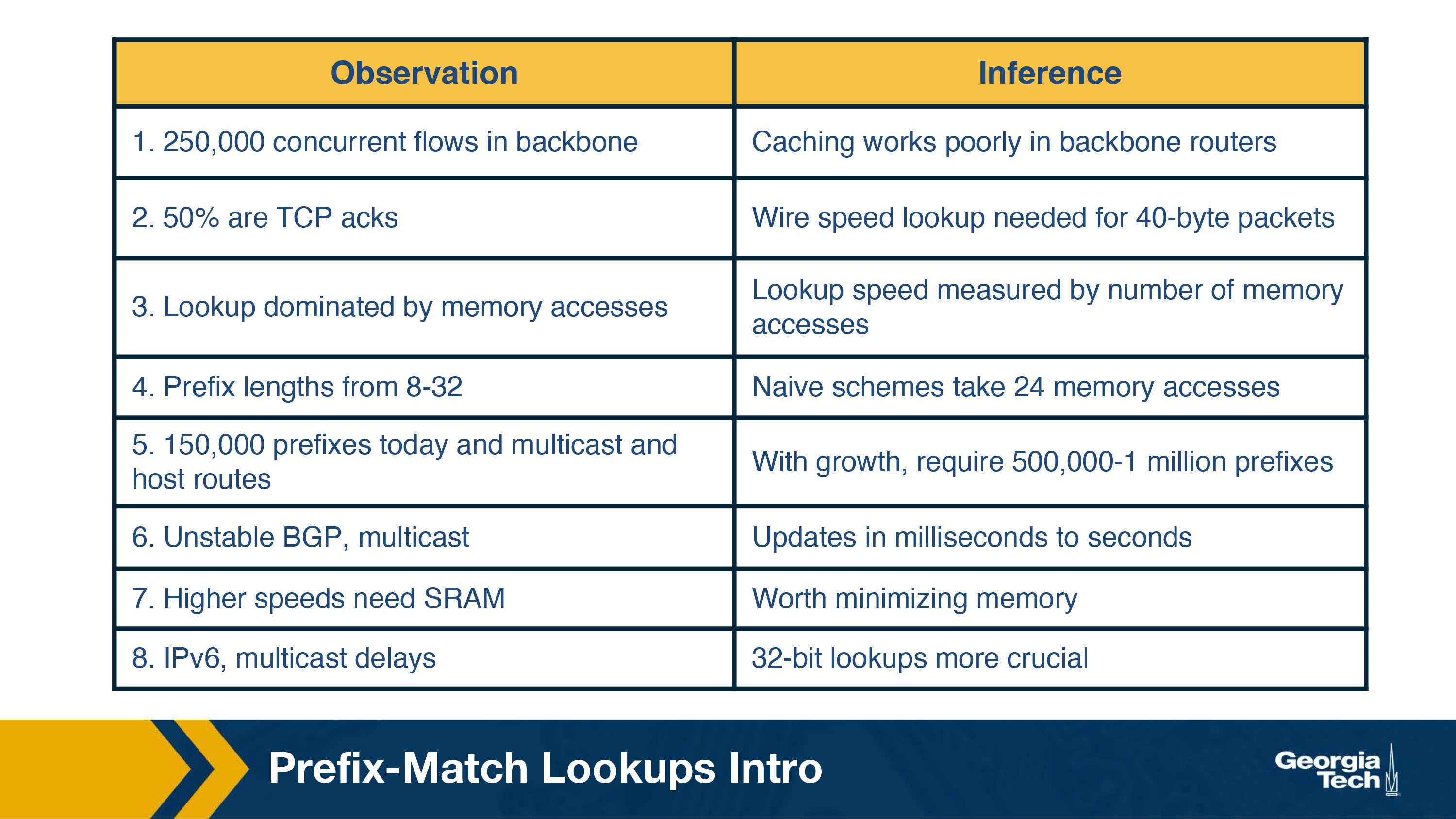
The main router performance metric is how quickly it can do a full lookup. There are four common problem areas:

1. A large amount of traffic is concurrent flows of short duration, making caching not very useful.
2. Lookup speed is important, the most costly part of that is accessing memory
3. An unstable routing protocol may result in more updates to the table and slower updates, adding milliseconds of time to the table update time.
4. Cost vs performance, really expensive memory is fast, cheaper memory is slower
   • how to decide which is which likely depends on application

Unibit Tries

Given this prefix db:

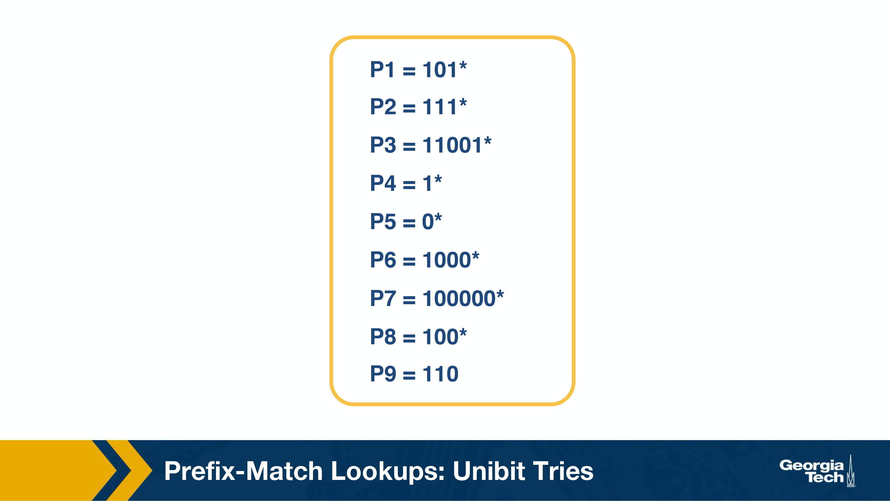
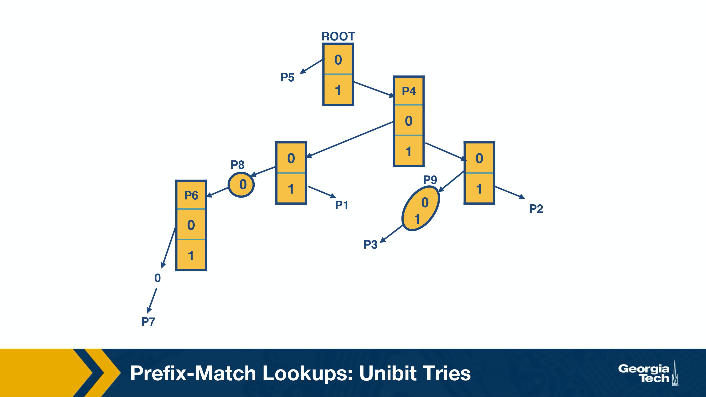
Results in this trie:

These are the steps we follow to perform a prefix match:

1. We begin the search for a longest prefix match by tracing the trie path.
2. We continue the search until we fail (no match or an empty pointer)
3. When our search fails, the last known successful prefix traced in the path is our match and our returned value.

Two notes:

1. If a prefix is a substring of another prefix, the smaller string is stored in the path to the longer (more specific prefix). For example, P4 = 1is a substring of P2 = 111, and thus P4 is stored inside a node towards the path to P2.

2. One-way branches. There may be nodes that only contain one pointer. For example, let’s consider the prefix P3 = 11001. After we match 110 we will be expecting to match 01. But in our prefix database, we don’t have any prefixes that share more than the first 3 bits with P3. So if we had such nodes represented in our trie, we would have nodes with only one pointer. The nodes with only one pointer each are called one-way branches. For efficiency, we compress these one-way branches to a single text string with 2 bits (shown as node P9).

Multibit Tries

Unibit tries are very efficient but it requires a large amount of memory accesses to achieve. For highspeed links it is not plausible to access memory that many times. Instead we use strides. A stride is the number of bits to check at each step.

So an alternative to unibit tries are the multibit tries. A multibit trie is a trie where each node has 2k children, where k is the stride. Next, we will see that we can have two flavors of multibit tries: fixed-length stride tries and variable-length stride tries.

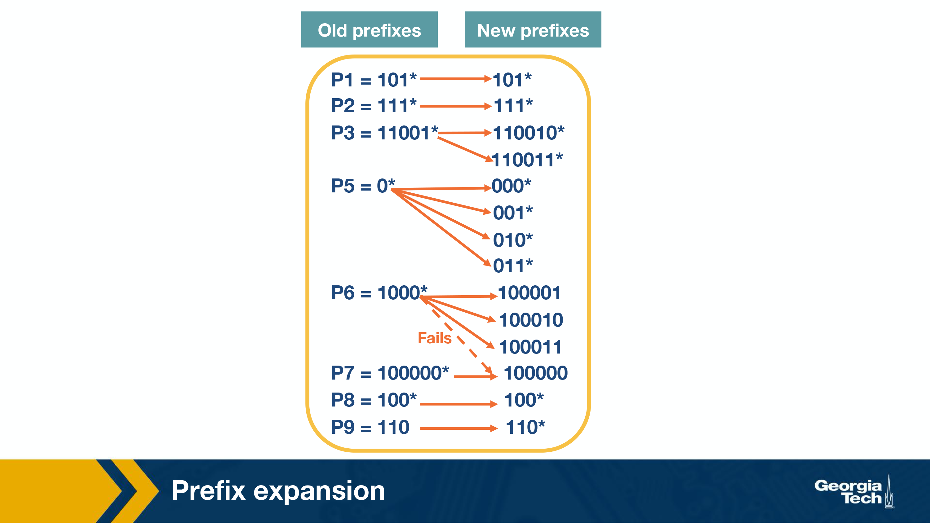
Prefix expansion

One quick problem you may run into with multibit, is if you have a stride length of 2, you could miss prefixes like 101* so this is handled via expansion:

Fixed Stride Example

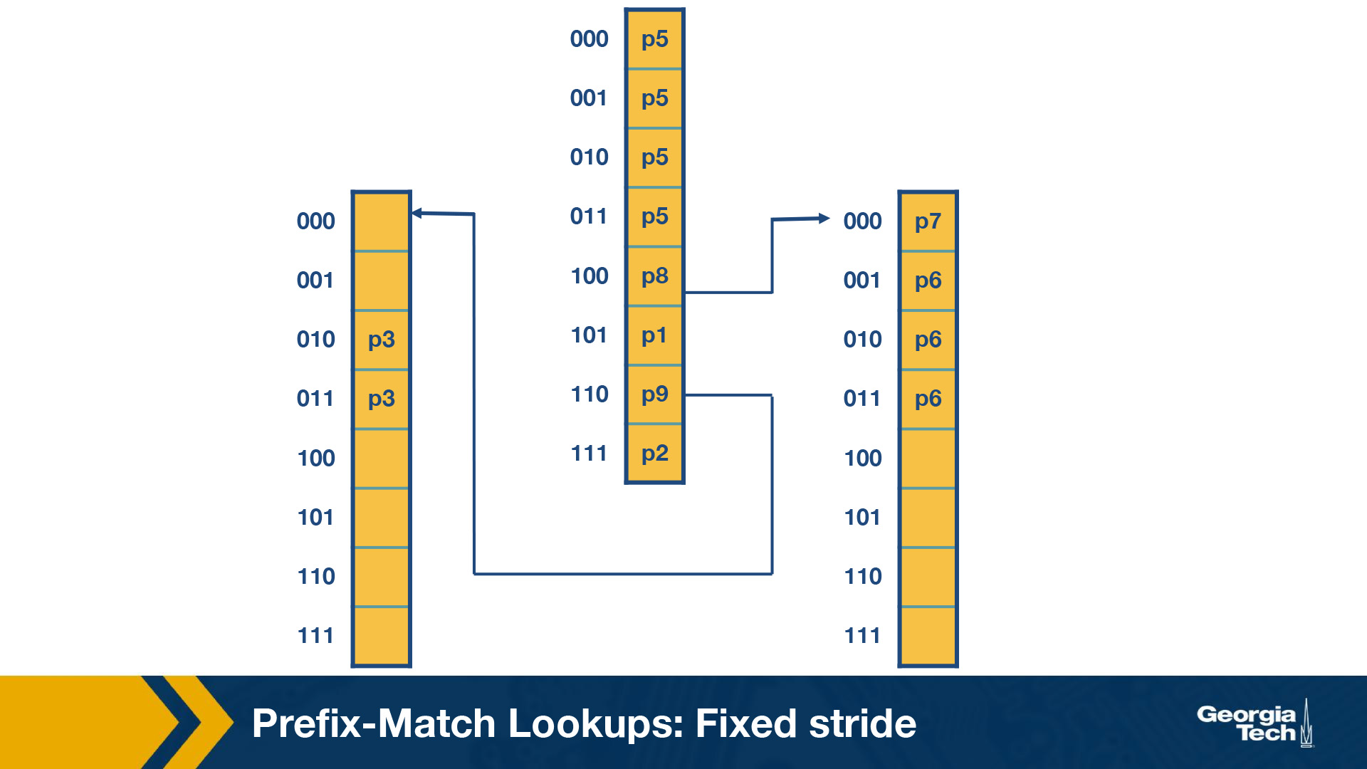
Using a fixed stride length of three, let’s do an example. Using the same database as the prior example.

Some key points to note here:

1. Every element in a trie represents two pieces of information: a pointer and a prefix value.
2. The prefix search moves ahead with the preset length in n-bits (3 in this case)
3. When the path is traced by a pointer, we remember the last matched prefix (if any).
4. Our search ends when an empty pointer is met. At that time, we return the last matched prefix as our final prefix match.

Variable Stride Length

Variable Stride length allows us to save memory and still get all of the addresses.

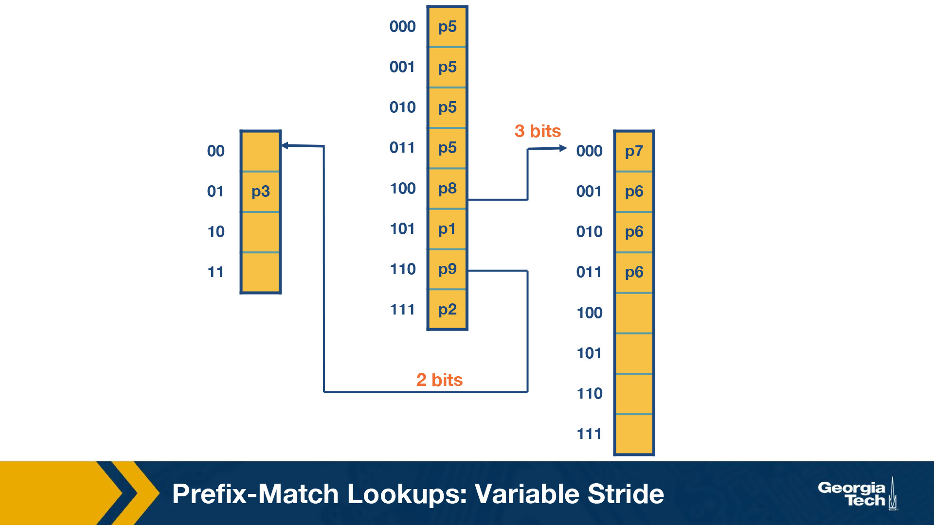
Some key points about variable stride:

1. Every node can have a different number of bits to be explored.
2. The optimizations to the stride length for each node are all done to save trie memory and the least memory accesses.
3. An optimum variable stride is selected by using dynamic programming

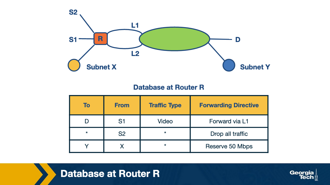
Packet Classification

We’ve talked aout prefix matching and how it attempts to solve the issue of an ever growing internet with many devices and many ip addresses.

What it doesn’t do is provide advanced features like paying attention to source addresses, tcp flags, etc.

Packet classification tackles those challenges.

Common examples:

1. Firewalls - Routers implement firewalls to filter inbound and outbound traffic based on a pre-determined set of policies.
2. Resource Reservation Protocols - To reserve bandwidth between a source and destination
3. Routing based on traffic type - If a certain type of traffic is more time sensitive, move it to the front of the queue

Simple Classifiers

• Linear Search - Perform a search through a rules database for every packet, works fine for simple rules, struggles at large amounts of rules
• Caching - Caching is usefule but has issues
  • Even an 80-90% cache rate still results in many searches
  • A 90% cache rate still has ~0.1 milliseconds of search, which is pretty slow in this context
• Passing Labels - Setup “Label Switched Paths” between sites,
  • Multiprotocol Label Switching (MPLS) and DiffServ use this
  • MPLS: router A does classification, and then all intermediate routers just read it and use it, instead of doing their own classification
  • DiffServ: Applies special markers at the edges to mark a packet for special quality-of-service

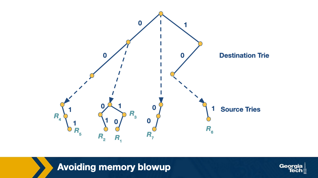
Fast Searching - Using Set Pruning Tries

Assume a two dimensional rule that only cares about source and destination IPs.

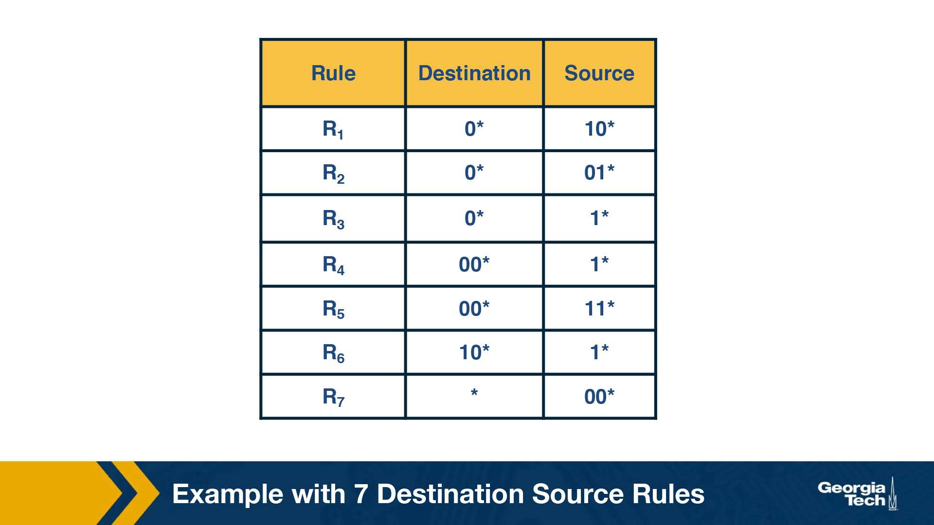
We can build a trie (similar to earlier in this section), where each leaf node is another trie

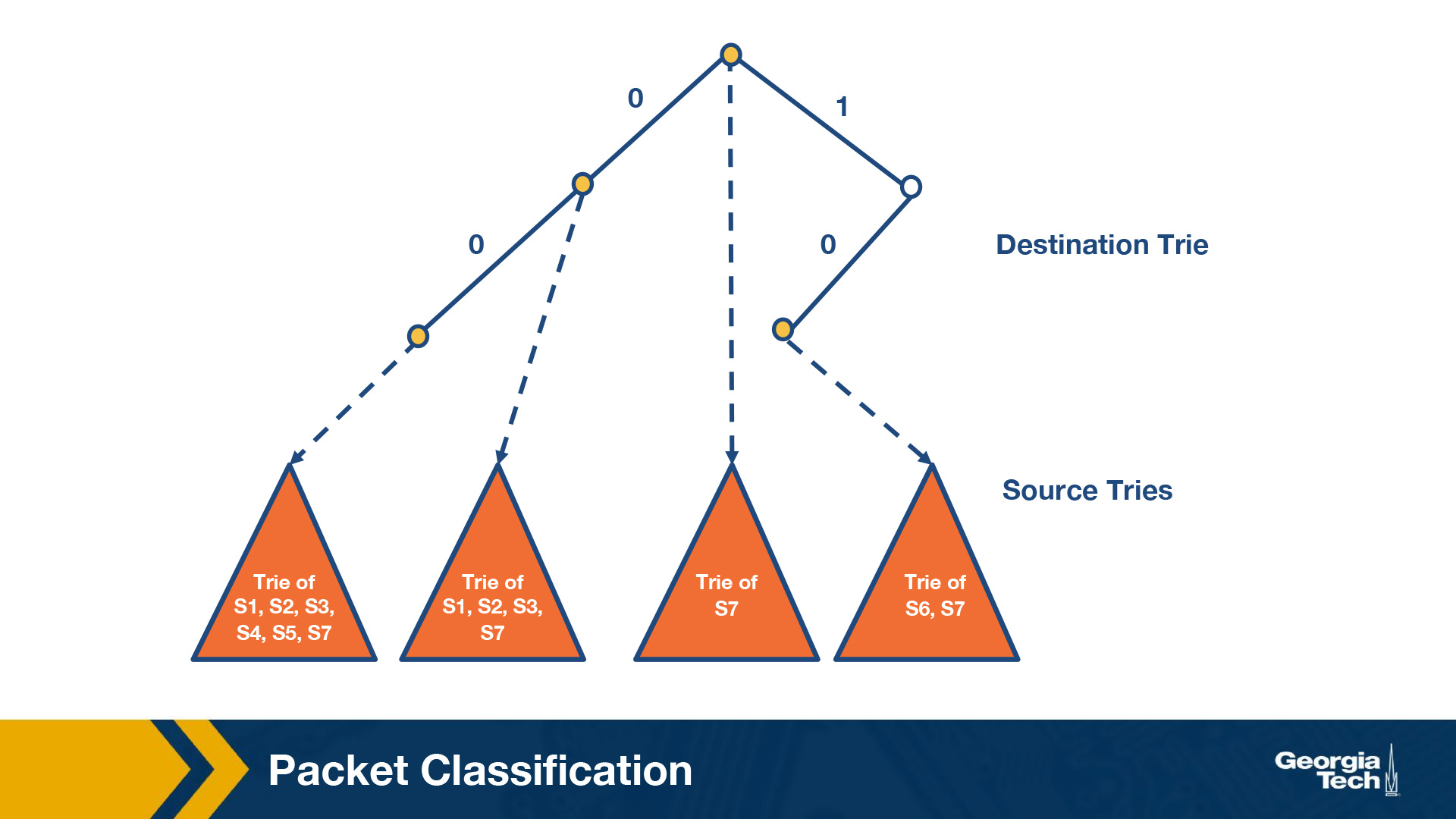
By S1, we denote the source prefix of rule R1, S2 of rule R2, etc. Thus for every destination prefix D in the destination trie, we “prune” the set of rules to those compatible with D. We first match the destination IP address in a packet in the destination trie. Then we traverse the corresponding source trie to find the longest prefix match for the source IP. The algorithm keeps track of the lowest-cost matching rule. Finally, the algorithm concludes with the least-cost rule. Challenge: The problem that we need to solve now is which source prefixes to store at the sources tries? For example, let’s consider the destination D = 00*. Both rules R4 and R5 have D as the destination prefix. So the source tries for D will need to include the source prefixes 1* and 11*. But if we restrict to 1* and 11*, this is not sufficient. Because the prefix 0*, also matches 00*, and it is found in rules R1, R2, R3, R7. So we will need to include all the corresponding source prefixes. Moving forward, the problem with the set pruning tries is memory explosion. Because a source prefix can occur in multiple destination tries.

Reducing Memory Using Backtracking

Set pruning has a high cost in memory to reduce time. So we can trade memory for time and try to solve this problem.

From the lecture:

The set pruning approach has a high cost in memory to reduce time. The opposite approach is to pay in time to reduce memory. Let’s assume a destination prefix D. The backtracking approach has each destination prefix D point to a source trie that stores the rules whose destination field is exactly D. The search algorithm then performs a “backtracking” search on the source tries associated with all ancestors of D. So first, the algorithm goes through the destination trie and finds the longest destination prefix D matching the header. Then it works its way back up the destination trie and searches the source trie associated with every ancestor prefix of D that points to a nonempty source trie. Since each rule is stored exactly once, the memory requirements are lower than the previous scheme. But, the lookup cost for backtracking is worse than for set-pruning tries.

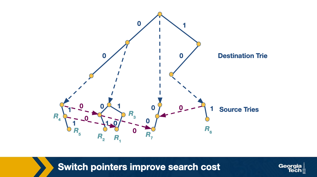
Grid of Tries

We’ve tried Backtracking (high time lower memory), and set pruning (memory explosion). Both fail for their own reasons.

Grid of tries approach takes backtracking and reduces wasted time by precomputing. When backtracking if there is a failure point in the source trie, we have a “switch pointer” which takes you directly to the next possible source trie containing a matching rule.

At places where there may be a failure to get to a matching rule, we can go directly to the next most likely place to find a rule, with precomputed switch pointers.

Scheduling

Now we talk about scheduling. Given a N-by-N crossbar switch with N input lines, N output lines, and N2 crosspoint we need to ensure that each input link is only connected to one output link at any given time and we want to maximize throughput by having the as many parallel routes open at one time as possible.

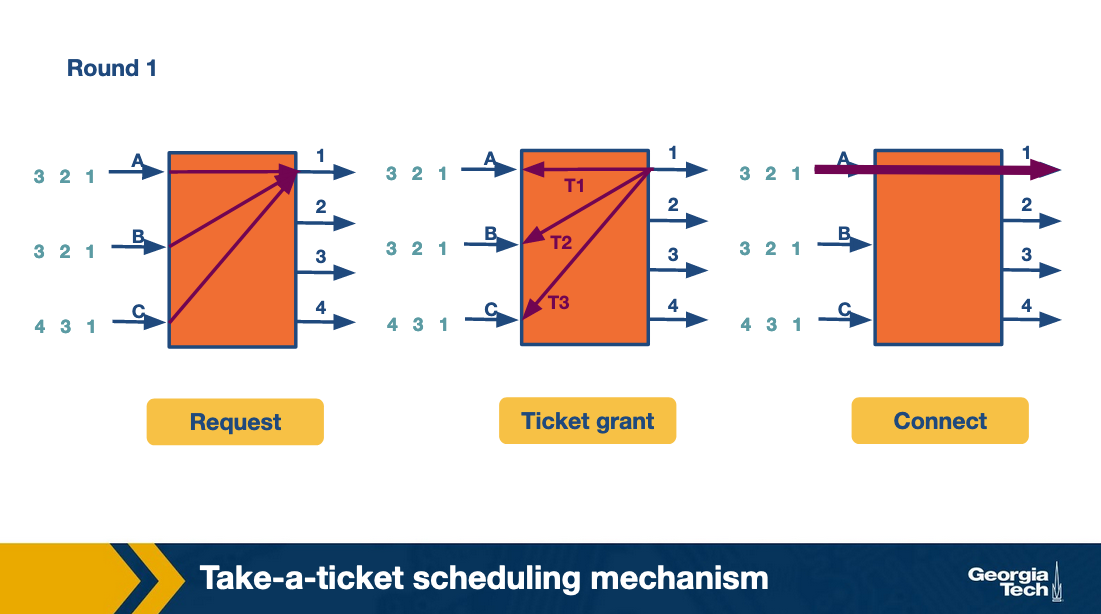
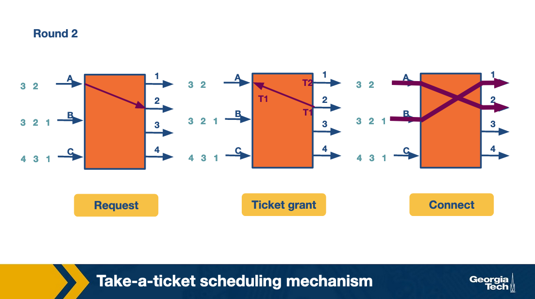
Take a Ticket Algorithm

Every output link has a queue, when an input link would like to use that queue it gets a ticket, and waits until it is called to send its packet and the route is opened.

Round 1:

Round 2:

Round 3:

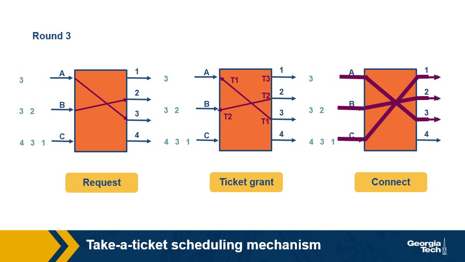
and here is an overview of how this all plays out:

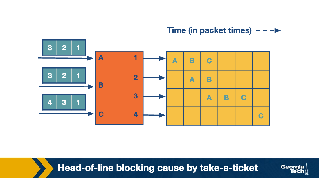
One thing to note here is that all of the other messages that are going to other nodes are blocked by the fact that they all wanted to go to output 1 first. This is “Head of line” blocking caused by take a ticket.

Avoiding Head of Line with Take a Ticket

Output Queuing

Given an N-by-N crossbar switch can we try to send to an output link without queuing? Then it would only need to block packets which are headed for the same destination. To do this the fabric must run N times faster than the input links.

A practical approach to this is the knockout scheme. It breaks up packets into fixed sizes k (which is smaller than N). Then if the fabric needs to only run k times as fast as an input link instead of N.

In some cases this can be broken and there are primitive switching rules to handle this.

• k = 1 and N = 2. Randomly pick the output that is chosen. The switching element, in this case, is called a concentrator.
• k = 1 and N > 2. One output is chosen out of N possible outputs. We can use the same strategy of multiple 2-by-2 concentrators in this case.
• k needs to be chosen out of N possible cells, with k and N arbitrary values. We create k knockout trees to calculate the first k winners.

The drawback of this approach is it is complex to implement.

Parallel Iterative Matching

This approach still allows queuing but in a way that avoids head-of-line blocking. It starts with taking each incoming link’s queue and breaking it into virtual queues for each output link.

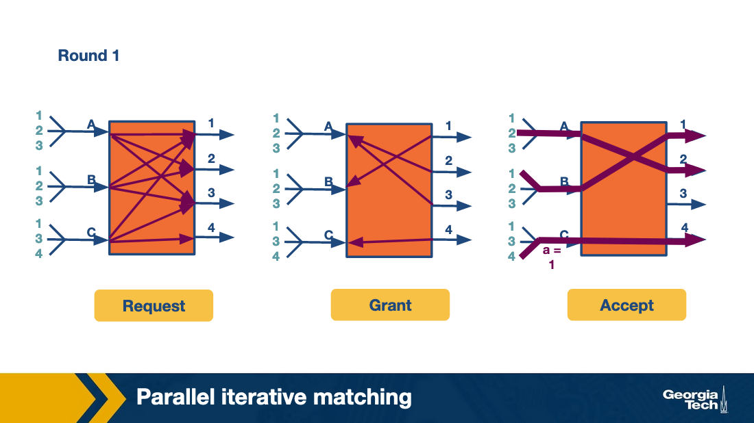
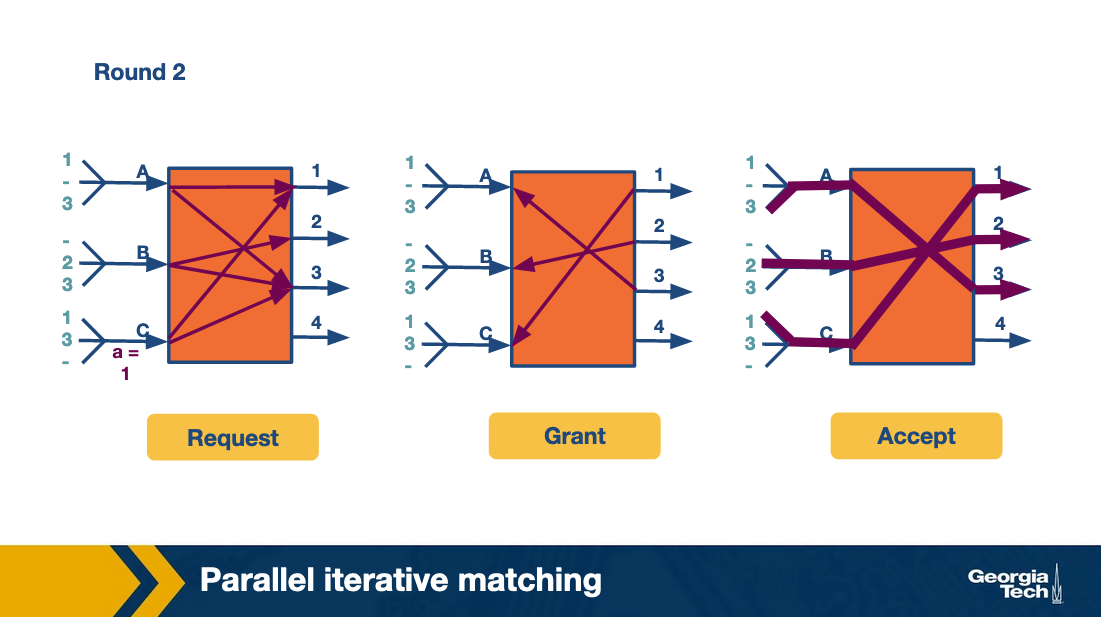
If an input receives multiple grants, it randomly picks between the two. This allows more packets to attempt to go through more quickly at the same time, and is more efficient than take-a-ticket.

Scheduling Intro

Busy routers rely on scheduling for routing updates, management queries, and data packets. Since linkspeeds are climbing over 40 gigabit, this needs to be done very quickly.

FIFO with tail drop

This is a simple first in first out queue, but if the queue is larger than its limit, the packets at the “tail” are dropped off.

Quality of Service

The FIFO approach has pretty bad quality of service with not guaranteed delivery due to dropping packets in the tail.

This is bad for the following reasons:

Router support for congestion

Congestion in the internet is increasingly possible as the usage has increased faster than the link speeds. While most traffic is based on TCP (which has its own ways to handle congestion), additional router support can improve the throughput of sources by helping handle congestion.

Providing QoS guarantees to flows

During periods of backup, these packets tend to flood the buffers at an output link. If we use FIFO with tail drop, this blocks other flows, resulting in important connections on the clients’ end freezing. This provides a sub-optimal experience to the user, indicating a change is necessary!

Fair sharing of links among competing flows

One way to enable fair sharing is to guarantee certain bandwidths to a flow. Another way is to guarantee the delay through a router for a flow. This is noticeably important for video flows – without a bound on delays, live video streaming will not work well.

Bit by Bit Round Robin

FIFO might drop packets. So we can use round robin to fix that. Pure round robin struggles though if one link has different packet sizes than the other, which might result in one link getting better service than the other.

Bit by Bit fixes this. The idea is that even though we can’t split packets up bit by bit, we can kind of do it virtually to help inform scheduling decisions. Using a lot of fancy math we can determine the round in which a packet finishes sending.

The Bit by Bit round robin then works by sending the packet which has the smallest finishing round number. Consider the following example:

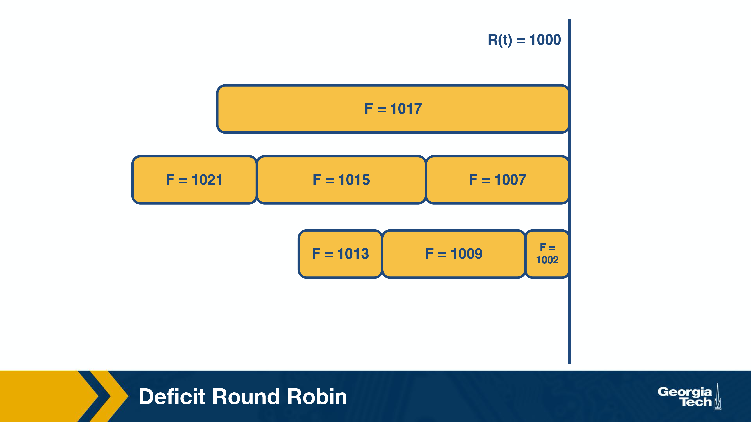
F is their finishing number, in their respective queues.

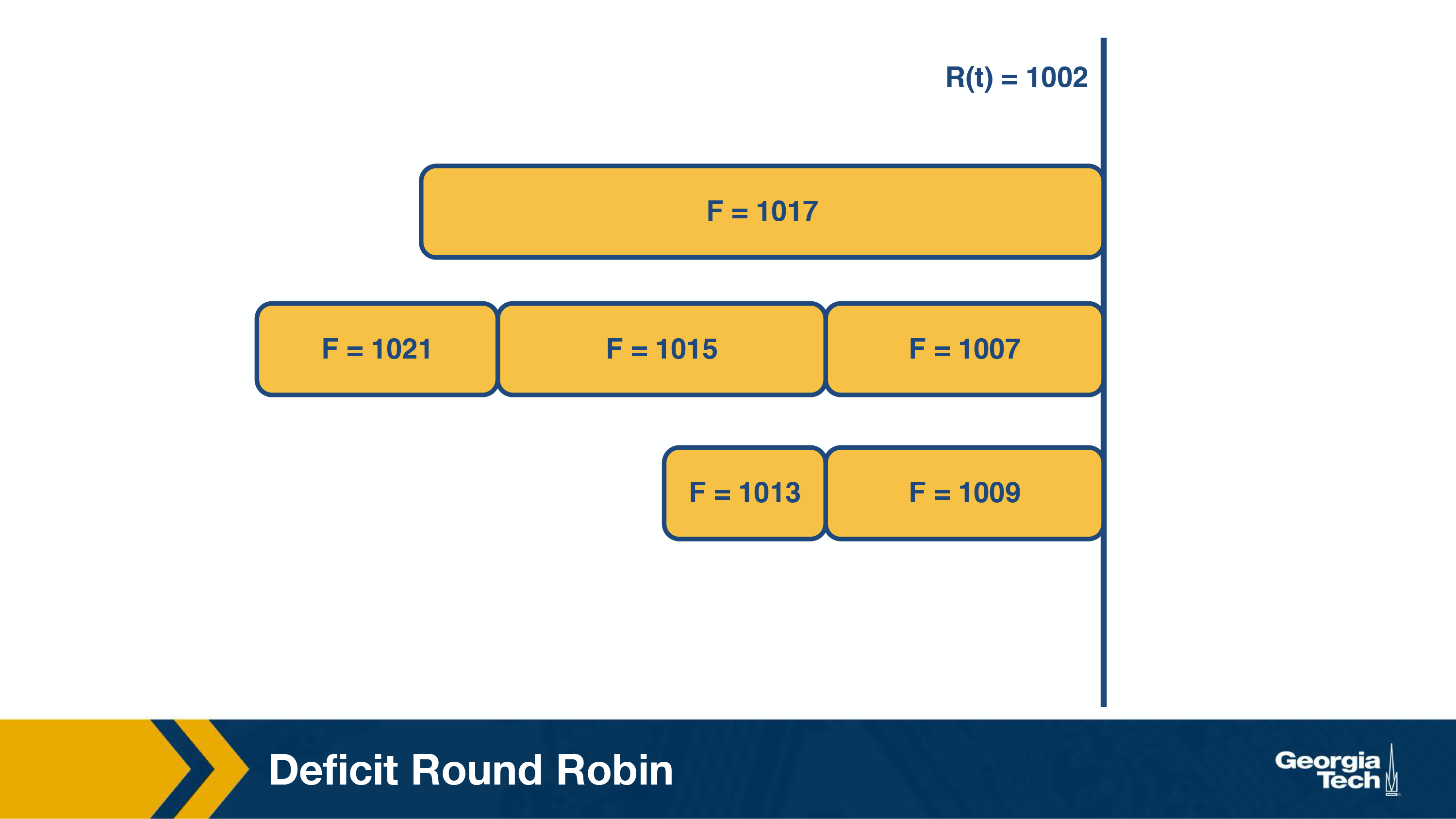
We can see F=1002 is sent first, because it had the earliers round finishing number. It was the “most starved” packet during the prior scheduling round.

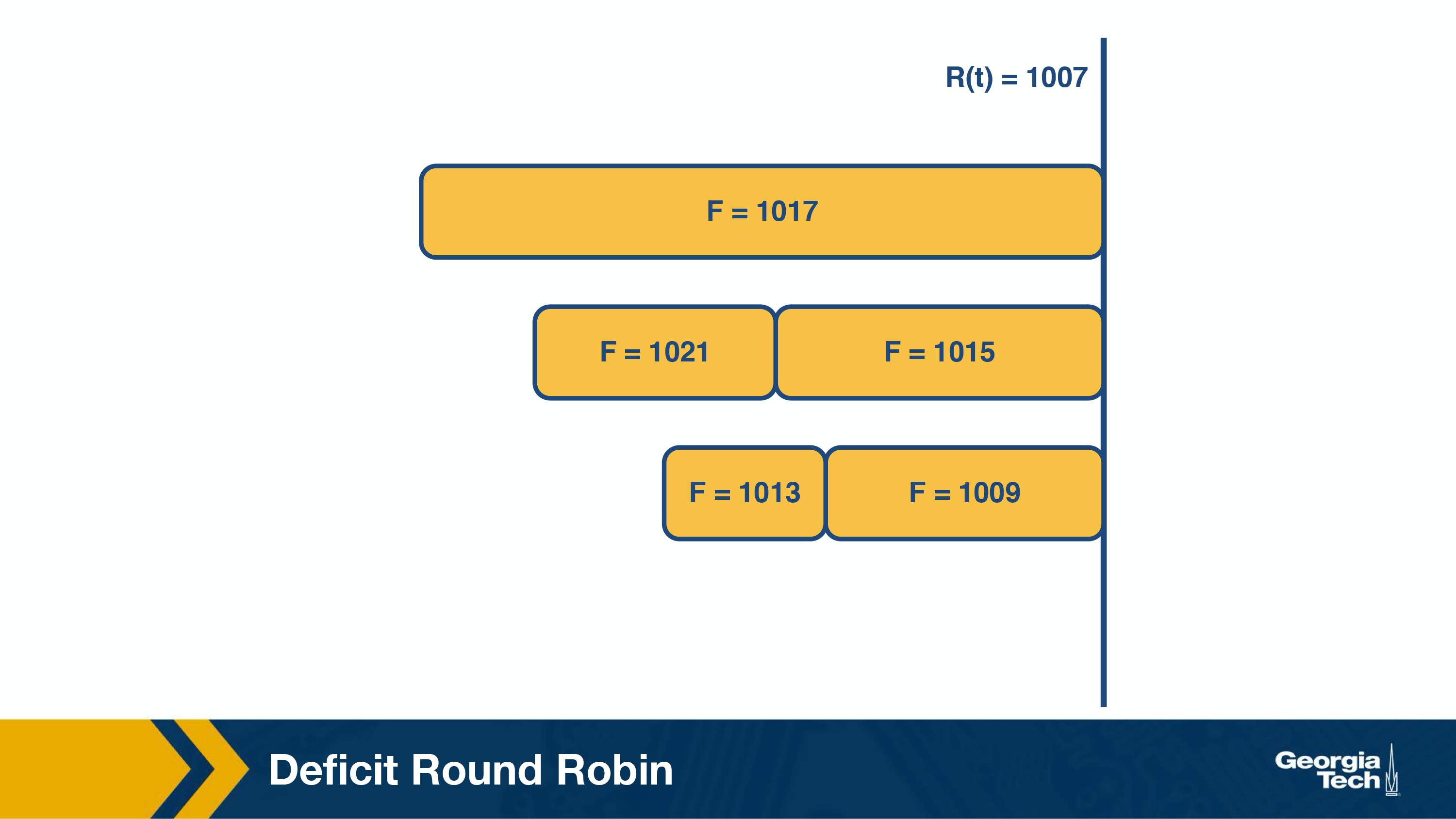
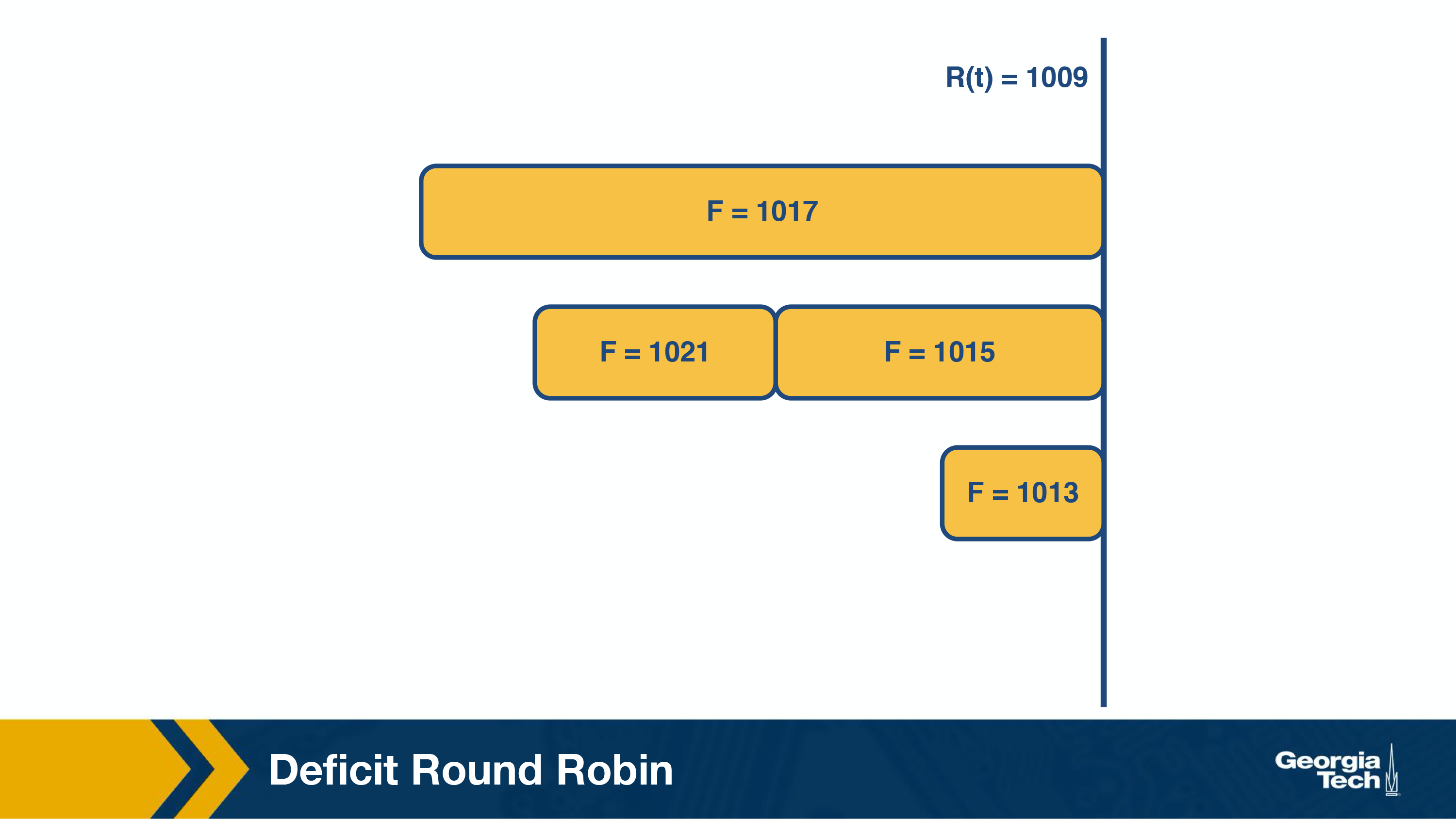
This is fair, but introduces new complexities. Specifically maintaining a priority queue becomes very expensive, and takes a long time, which isn’t feasible at gigabit speeds.

Deficit Round Robin

Round robin guaranteed delay and bandwidth fairness, but many applications only care aobut bandwidth fairness. So a simple constant-time round robin could get that done much more simply.

We assign a quantum size, Qi, and a deficit counter, Di, for each flow. The quantum size determines the share of bandwidth allocated to that flow. For each turn of round-robin, the algorithm will serve as many packets in the flow i with size less than (Qi + Di). If packets remain in the queue, it will store the remaining bandwidth in Di for the next run. However, if all packets in the queue are serviced in that turn, it will clear Di to 0 for the next turn.

Consider the following:

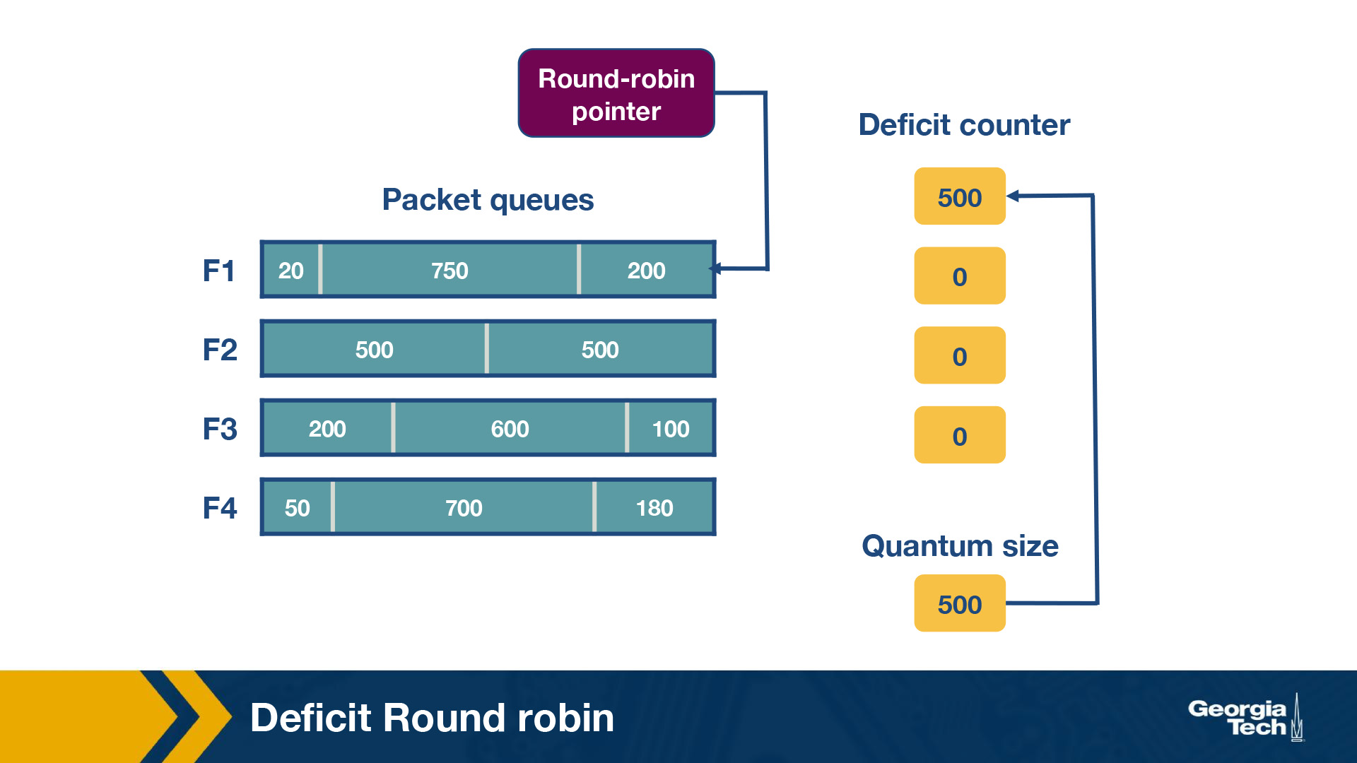
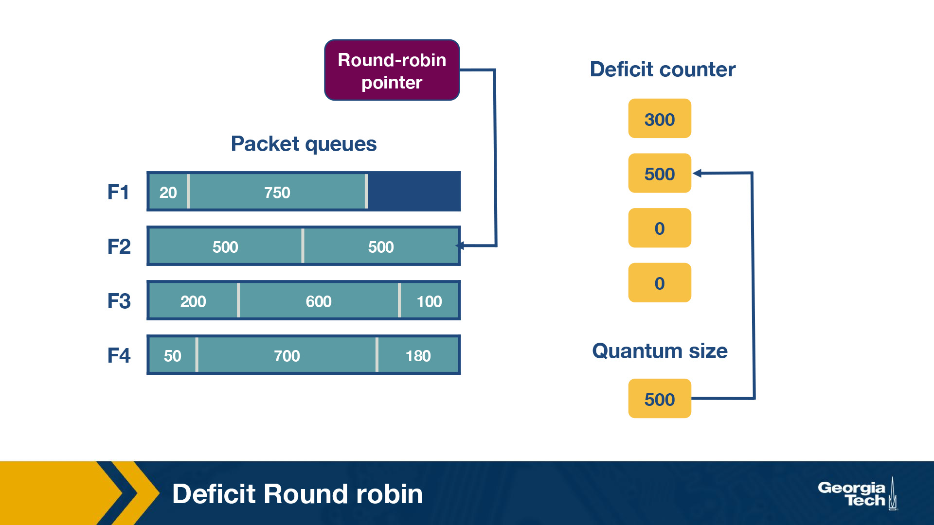
In this router, there are four flows – F1, F2, F3, and F4. The quantum size for all flows is 500. Initially, the deficit counters for all flows are set to 0. Initially, the round-robin pointer points to the first flow. The first packet of size 200 will be sent through. However, the funds are insufficient to send the second packet of size 750. Thus, a deficit of 300 will remain in D1. For F2, the first packet of size 500 will be sent, leaving D2 empty. Similarly, the first packets of F3 and F4 will be sent with D3 = 400 and D4 = 320 after the first iteration. For the second iteration, the D1+ Q1 = 800, meaning there are sufficient funds to send the second and third packets through. Since there are no remaining packets, D1 will be set to 0 instead of 30 (the actual remaining amount).

Token Bucket

Sometimes we want to limit flows of certain data types without having to put them into another queue.

Token bucket shaping can accomplish this through things like limiting burstiness of flow by limiting the average rate, and limiting the burst maximum size allowed.

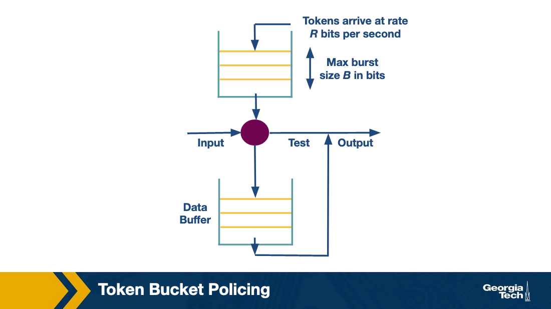
If a packet comes and needs to hit the bucket, the bucket has to have enough available tokens, otherwise it fails. That’s how you limit burst.

The problem with this is only one queue per flow. If a flow has a full token bucket it may block other flows. Token policing solves this.

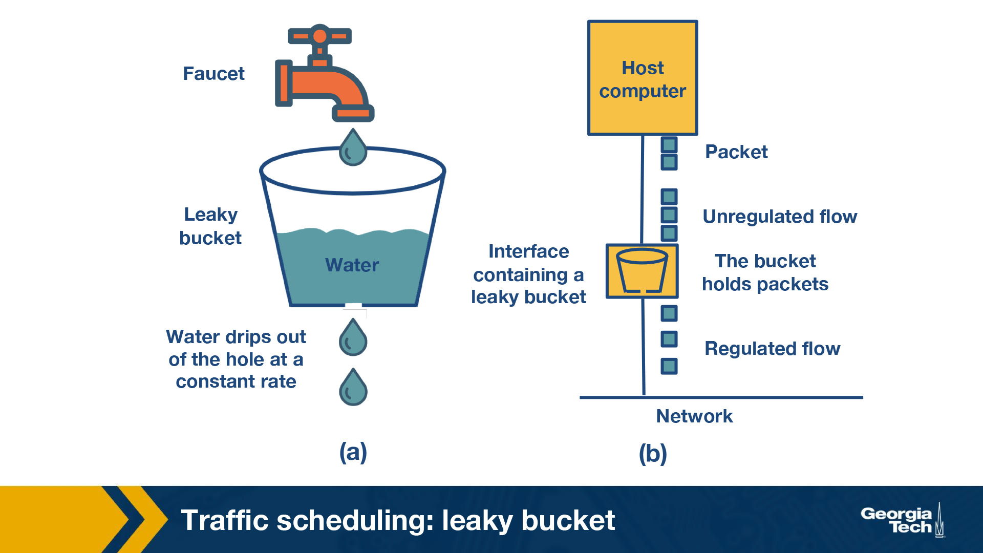
Leaky Bucket (Token Policing)

Policing and shaping both help limit the output of a link but in different ways.

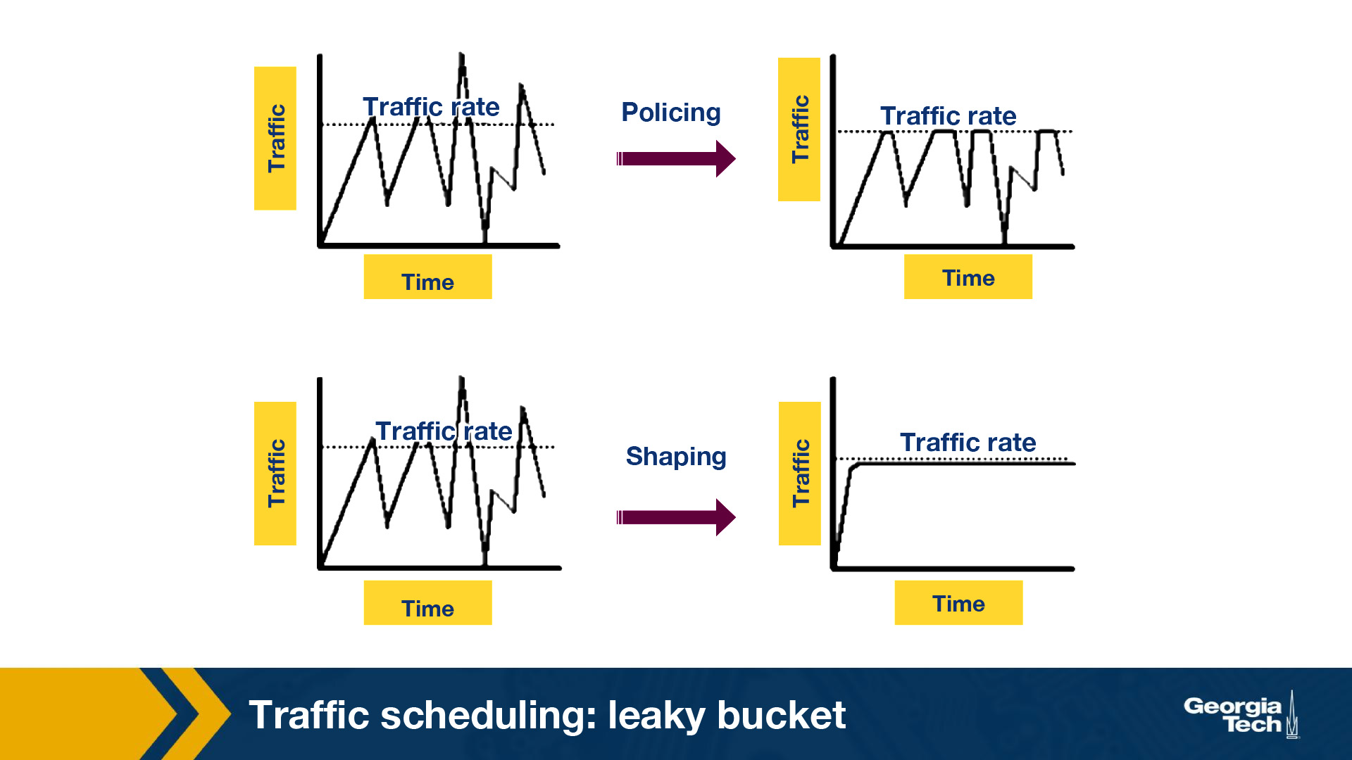
• Policer: When the traffic rate reaches the maximum configured rate, excess traffic is dropped, or the packet’s setting or “marking” is changed. The output rate appears as a saw-toothed wave.
• Shaper: A shaper typically retains excess packets in a queue or a buffer, and this excess is scheduled for later transmission. The result is that excess traffic is delayed instead of dropped. Thus, the flow is shaped or smoothed when the data rate is higher than the configured rate. Traffic shaping and policing can work in tandem.

Leaky bucket refers to the Token Bucket implementation with a constant output rate. If a packet were to make a bucket overflow it is discarded, but the same time things aren’t sent in burst, but at a constant “leak” rate.

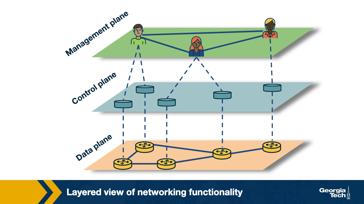
Lesson 7 - Software Defined Networking

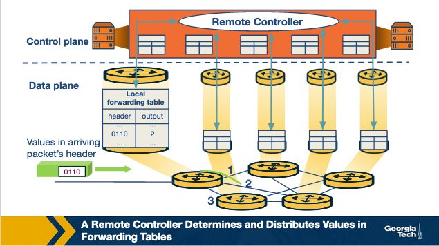
Software Defined Networking (SDN) was borne of the need to separate the control plane from the data plane.

Why did SDN arise?

There was a need to make computer networks more programmable, because there is a diversity of equipment on every network, and many proprietary technologies.

Diversity of Equipment

Routers, switches, firewalls, network address translators, server load balancers, intrusion detection systems, oh my! These are just some of the types of devices that get put on a network.

Even with a centralized network controller, there are so many different protocols and interfaces that need support, it creates quite a lot of work to support it.

Proprietary Technologies

Switches and routers often ran proprietary software. Likely done to encourage people to buy all of a certain brand, but in instances where that’s not feasible for one reason or another then something has to deal with those differences.

SDN looks to fix all of these issues with ✨software✨. It does this by separating tasks. Specifically separating the control plane and the data plane.

History of SDNs

The history of SDN can be divided into three phases:

1. Active networks
2. Control and data plane separation
3. OpenFlow API and network operating systems

Active Networks

From the mid 1990s until the early 2000s the internet of course exploded. This required new porotocols which were to be created by the Internet Engineering Task Force (IETF). This process sucked and then other things sprung up to fill the holes.

It led to the growth of active networks which used wanted a programming interface which exposed many resources and allowed customization of functionalities for subsets of packets passing through the network. This was opposite to the belief that a simple network core was important to internet success.

There were two prevalent programming models in active networking with the difference being where code is executed:

1. Capsule Model - carried in band pockets
2. Programmable router/switch model - established out of band mechanisms

The main pushers of active networks was

• Reduction in computation cost, enables more processing
• Advancement in programming languages, enabled things that were previously not possible, of if they were possible, were unsafe
• Advances in rapid code compliation and formal methods
• Funding from DARPA (DARPA just keeps showing up)

The main pullers of active networks was:

• Network service providers were frustrated with long timelines to deploy new network services
• Third parties wanting to get more control on an individual level
• Unified control over middleboxes

These pulls are similar pulls to the current pulls for SDN.

Active networks made three major contributions to CDNs:

• Programmable functions in the network to lower the barrier to innovation
  • Active networks were one of the first to use the idea of programmable networks to overcome the slow speed of innovation in computer networks.
  • Lots of focus was on programming the control plane, but active networks tried to add some to the data plane
  • This is similar to OpenFlow and other SDN ideas that are being used
• Network virtualization, the ability to demultiplex software programs based on packet headers
  • Active networking produced a framework that described a platform that would support experimentation, this led to virtualization
• Unified Architecture for middlebox orchestration
  • Control over middleboxes was never fully realized in Active networks but some of its research is benefitting network function virtualization

Active Networks main reason for not beocming main stream is due to the fact that it was too ambitious. It required people to program in Java, which was not guaranteed, and did not have security as a focus from the beginning, which scared people.

Control and data plane separation

Control and data plane separation was from around 2001 to 2007. Network operators were desperate to have better management tools of their traffic as the network popularity exploded.

It was identified that many of the main issues had to do with the tight coupling of the control and data planes.

The main pushers of control and data plane separation were:

• Higher link speeds in backbone networks
• Internet service providers had a difficult time meeting the increased reliability and new services
• Servers had substantially more memory and processing resources than things made even 1 or 2 years earlier
• Open source routing software lowered the barrier to creating centralized routing controllers

These pushes resulted in:

• Open interface between control and data planes
• Logically centralized control of the network

It was different from active networking in the following ways:

• Focused on spurring innovation by and for network administrators
• Emphasized programmability in the control domain rather than the data domain
• Worked towards network-wide visibility and control rather than device level

The main pullers of control and data plane separation were:

• Selecting between network paths based on current traffic load
• Minimizing disruptions during planned routing changes
• Redirecting/dropping suspected attack traffic (firewall)
• Allow customers more control over traffic flow
• Offering value add services for virtual private network customers

Most of this work was completed within an ISP, with not much cross ISP interfacing. There were a couple concepts which were taken into SDN design:

1. Logically centralized control using an open interface
2. Distributed state management

People thought this was a bad idea because what if the controller failed. In addition to this people were nervous about distributed network maps instead of the routers knowing the whole picture.

OpenFlow API and network operating systems

This took place during 2007 to 2010.

The OpenFlow API was borne fromm an interest in the idea of network experimentation at scale. It balanced fully programmable networks with real world deployments.

It was built on existing hardware but enabled more functions that prior controllers. This dependency was based on hardware flexibility, but it enabled immediate deployment.

OpenFlow switches follow this:

• Each switch contains a table of packet-handling rules
• Each rule has a pattern, list of actions, set of counters, and priority

Once a packet is recieved it determines the highest priority matching rule, performas the action associated with it, and increments the counter

The main pushers of this technology were:

• Switch chipset vendors had already started to allow programmers to control some forwarding behaviors
• Allowed other companies to build their own switches without making a data plane
• Enabling OpenFlow was easy to deploy based on a simple firmware upgrade

The main *pullers of this technology were:

• OpenFlow was meeting the need of conducting large scale experimentation on network architectures
• OpenFlow was useful in data-center networks that had a need to manage network traffic
• Companies started investing more in programmers for cotnrol programs and less on proprietary hardware, allowing smaller players to get in the game

OpenFlow’s Key Effects:

• Generalized network device and functions
• Provided a vision of a network operating system
• Distributed state management techniques

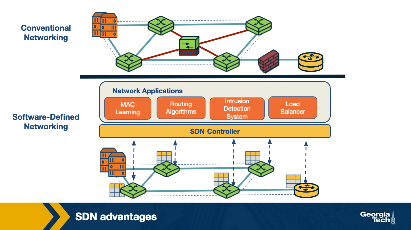
Separating the Data Plane and the Control Plane

SDN is different from the traditional networking approaaches because it separates the control and data plane.

The reasons for this separations are:

• Independent evolution and development
  • Routing and forwarding are tied to a single piece of hardware, meaning the only easy time to upgrade, is when you do the whole thing. By separating them, routing can grow while forwarding stays the same, and vice versa. Coupling makes things difficult.
• Control from high-level software program
  • Using software to compute forwarding tables means higher order programs can control router behavior. Not being attached to the forwarding plane makes this simpler.

It’s best for both planes that they go their separate ways :)

This then enables:

1. Data Centers, large data centers with oodles of compute, but using that compute can become even more difficult if you’re rigidly attached to the forwarding hardware
2. Routing, separating the two allows more complex routing
3. Enterprise networks. SDN can imporve sescurity of networks by protecting from things like DDoS by simply dropping traffic at strategic locations
4. Research networks. You can colocate research and production networks, allowing for experimentation on live traffic without interfering with said live traffic

Traditional Router:

SDN approach:

SDN Architecture

The main components af an SDN network are:

• SDN controlled network elements - The infrastructure layer is responsible for the forwarding of traffic in a network based on rules from the SDN control plane
• SDN controller - Logically centralized entity that acts as the interface between network element and network control applications
• Network control applications - Programs that manage the underlying network by observing network elements through the SDN controller

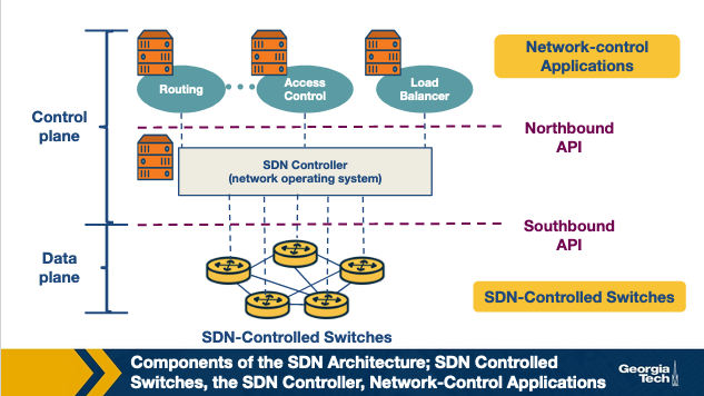
Four defining features

The four defining features of SDN architecture are

• Flow-based forwarding
• Separation of data plane and control plane
• Netowrk control functions
• A programmable network

Flow-based forwarding

The rules for forwarding packets can be computed based on any number of header values from various layers. This differes from the prior approach in which only the destination IP address determined the forwarding of a packet. OpenFlow allowed up to 11 header field values to be used

Separation of data plane and control plane

SDN controlled switches only operate on the data plane executing rules in the flow tables, created and managed by entirely separate servers

Network control functions

The SDN control plane usually runs on multiple servers for increased performance and availability. It also consists of two componetns

1. Controller
2. Network applications

The controller maintains up to date network state info and provides it to network control applications. This is used by the applications to monitor and control network devices

A programmable network

Since you have the network-control applications which act as the “brain” of the SDN control plane you can do things like network management, traffic engineering, security, automation, etc. Something like determining the end-to-end path between sources and destinations in the network using Dijkstra wink wink.

SDN Controller Architecture

The SDN controller is a part of the SDN control plane. It acts as an interface between the network elements and the network-control applications.

SDN Controller Layers

• Communication Layer - Communicating between the controller and network elements
• Network-wide state-management layer - Stores information of network-state
• Interface to the network-control application - communicating between controller and applications

Communication Layer

This layer has a protocol which the SDN controller and the network controlled elements communicate. This protocol is used so that network devices can send things like new device joining, heartbeat indicators, etc. The communication between SDN controller and the controlled devices is the “southbound” interface. OpenFlow does this.

Network-wide state-management layer

This is pretty self-explanatory, everything that has to do with the network state that is managed by the controller. State of hosts, links, switches and copies of flow tables of various switches. This is what is used by the control plane to configure flow tables.

Interface to the network-control application

This layer is the “northbound” interface and how the SDN controller interacts with network-control applications. Network control applications read/write network state, flow tables, etc in the state-management layer. The SDN controller can also notify applications of changes in state as well.

Generally these SDN controllers are implemented in a distributed fashion in order to achieve fault tolerance, high availability and efficiency.

Lesson 8 - Software Defined Networking (Part 2)

Again, CDN is a more independently layered approach to Routing

SDN Advantages compared to Traditional

1. Shared Abstractions. Middlebox services (or network functionalities) can be programmed easily since the abstractions provided by the control platform and network programming langauges can be shared
2. Consistency of same network information. All network apps have the same global view leading to more consistent policy decisions while reussing control plane modules
3. Locality of functionality placement. Previously middlebox locations were strategic decisions and often big constraints. With SDN middleboxes can be whereever
4. Simpler Integration. It’s easier to integrate to SDN things than traditional proprietary boxes

SDN Landscape

Again SDN can be viewed as layers:

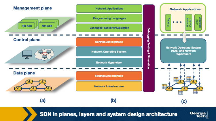
(a) is plane-oriented view, (b) is the SDN layers, (c) is a system design perspective.

SDN Architecture

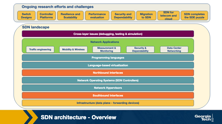
Infrastructure

Instead of needing routers with switching and control plane, physical networking equipment only needs to do simple forwarding. All logic comes from a centralized control system.

Southbound Interfaces

Communications between control and forwarding elements (switches) is on the southbound interface. These APIs are tightly coupled with the forwarding elements. The most popular implementation is OpenFlow.

Network Virtualization

A complete virtualization of a network needs to support arbitrary network topoligies and addressing scheemes, similar to the computing layer. VLAN, NAT and MLPS can provide this full virtualization but this is a box-by-box basis configuration and there is no unifying abstraction to do this in a global manner. So this is one thing that takes a long time still.

Network Operating Systems

These operating systems abstract away many low level things like distribution among routing elements, allowing developers to focus on more complex applications. Examples are OpenDayLight, OpenContrail, etc

Northbound Interfaces

The Northbound interface is how the controller and the network applications talk. There is no set standard for this interface, but one key difference is it’s usually purely software to software communication, unlike the southbound interface. Popular examples are Floodlight, Trema, NOX, ettc.

Language-based virtualization

Allowing network devices to be interacted with via many ways at different levels of abstraction. Takes away device communication complexity without compromising security.

Network programming langauges

By having high level programming laguages in SDNs it gives more abstractions to make development more modular, things more reusable and do away with device specific low-level configurations.

Network applications

The functionalities implementing control plane logic and translates to commands in the data plane. There is avery wide range of options for these applications, doing things like routing, load balancing, security enforcement, and more.

SDN Infrastructure Layer

SDN infrastructure contains routers, switches, and appliance hardware.

The physical devices have no embedded intelligence, as it’s delegated to the central control system, the Network Operating System (NOS). These are built on open-souce interfaces to encourage improvements and growth to the networking sphere.

A data plane devices forwards packets, a controller is a software stack running on commodity hardware. The most widely used data plane device is a model derived from OpenFlow. There’s a pipeline of flow tables where each entry should have a matching rule, actions to be executed on matching packets, counters keeping statistics of matching packets.

In OpenFlow device

1. Packet arrives
2. Lookup starts, either matches with rule or misses
3. Resolve
   1. forward to outgoing port
   2. encapsulate and send to controller
   3. drop packet
   4. send to normal processing pipeline
   5. send to next flow table

SDN Southbound interrfaces

Sounthbound interfaces are the APIs separting the control plane and the data plane. Since switch hardware takes time to design and engineer, this has settled on a standard protoocol of OpenFlow.

The OpenFlow protocol supports three info sources:

1. Event based messages sent by forwarding devices to the controller when there is a link or port change
2. Flow statistics generated by forwarding devices and collected by controller
3. Packetss sent by forwarding devices when they don’t know what to do with them

The controller and network operating system uses this flow of information to make decisions and maintain states/maps/flow charts.

SDN Controllers - Centralized vs Distributed

The core controllerr functions are:

• Topology
• Statistics
• Notifications
• Device Mangement
• Shortest Path forwarding
• Security mechanisms

Centralized controllers

A single entity manages all forwarding devices in the network. This has a single point of failure and can have a hard time scaling. Some enterprise class networks and data centers use archietctures that allow this and use giant mult-threaded designs alllowing for large amounts of throughput even on a single server.

Distributed controllers

Distributed controlling can scale to meet practically and requirement, because it’s built in to the design to scale as needed. It can be a centralized cluster of nodes, or a physically distributed set of elements. If a provider has multiple data centers, they might even do a hybrid where each center has a cluster, but they talk physically in a physically distributed manner.

Open Network Operating System

This is an example of a distributed SDN control platform.

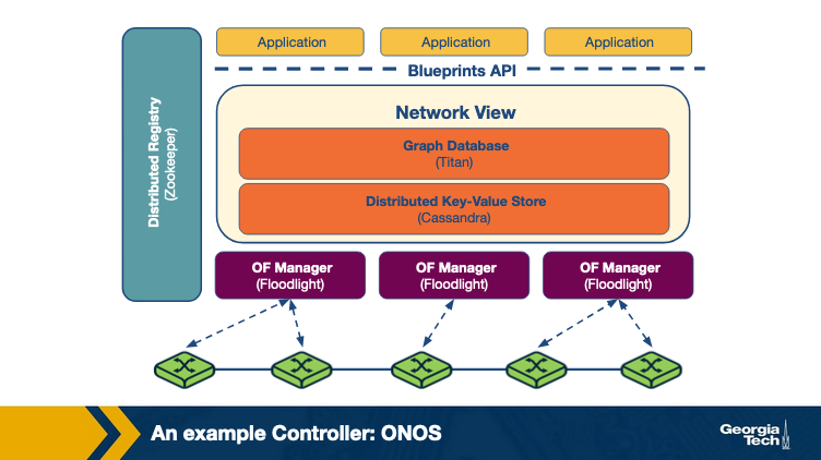
ONOS has several instances running in a cluster. The network state is shared across these instances by maintaining a global view. The view is made with network topology and state information.

Forwarding and policy decisions come from the view, OpenFlow managers recieve changes, and switches are programmed.

Titan is a graph database and Cassandra a distributed key-value store work together to create the view. They interact with this using the Blueprints Graph API.

The ONOS archictecture can scale out and offers fault tolerance. In ONOS there is a master controller for a group of switches, and the propagation of state changes is handled solely by the master instance of that switch. This is distributed by adding more instances, reducing number of switches to contoller instances.

Fault tolerance is achieved by handling failures via election, where if the master controller of a switch fails, the rest of the ONOS instances it is connected to fomr on consensu on who the new master should be for each of the switches that were failed.